PROJECTS WITH APPLICATIONS OF DIFFERENTIAL …

1 PROJECTS with APPLICATIONS OF DIFFERENTIAL equations AND MATLAB. David Szurley Francis Marion University Department of Mathematics PO Box 100547. Florence, SC 29502. I. INTRODUCTION. DIFFERENTIAL equations (DEs) play a prominent role in today's industrial setting. Many physical laws describe the rate of change of a quantity with respect to other quantities. Since rate of change is simply another phrase for derivative, these physical laws may be written as DEs. For example, Newton's Second Law of Motion states that the rate of change of momentum of an object is equal to the sum of the imposed forces. Normally this is written as F ma m , where F represents the total imposed force. However, if we let x denote the position of the object, then this may be rewritten as F m&x&.

2 Hence, Newton's Second Law of Motion is a second-order ordinary DIFFERENTIAL equation. There are many APPLICATIONS of DEs. Growth of microorganisms and Newton's Law of Cooling are examples of ordinary DEs (ODEs), while conservation of mass and the flow of air over a wing are examples of partial DEs (PDEs). Further, predator-prey models and the Navier-Stokes equations governing fluid flow are examples of systems of DEs. Many introductory ODE. courses are devoted to solution techniques to determine the analytic solution of a given, normally linear, ODE. While these techniques are important, many real-life processes may be modeled with systems of DEs. Further, these systems may be nonlinear. Nonlinear systems of DEs may not have exact solutions . However, we still desire some type of solution.

3 There are many numerical techniques to obtain an approximation to the solution of a DE or system of DEs. Many scientific packages contain library commands to numerically approximate the solution of these. In particular, MATLAB contains the ode45 command which will numerically approximate the solution to a system of ODEs using a medium order method. Thus, the scientific package MATLAB may be used to explore DEs modeling real-world APPLICATIONS that are more complicated than the DEs presented in a typical introductory course. Using MATLAB also has the advantage that the internal command guide may be used to create graphical user interfaces (GUIs) to help facilitate this exploration. The GUIs ensure that the students are not bogged down with reading and understanding MATLAB code.

4 In this paper, we will discuss how to use MATLAB to simulate the solution to DEs. Then PROJECTS the author has assigned involving real-world APPLICATIONS of DEs will be described. One project models the industrial process of film casting while the other models the conduction of heat within a one-dimensional rod. Similar PROJECTS will also be briefly described. Finally, student feedback from the PROJECTS will be given. 234. II. SIMULATING solutions TO ORDINARY DIFFERENTIAL equations IN. MATLAB. MATLAB provides many commands to approximate the solution to DEs: ode45, ode15s, and ode23 are three examples. Suppose that the system of ODEs is written in the form y' f t , y , where y represents the vector of dependent variables and f represents the vector of right-hand- side functions.

5 All of the commands ( , ode45) require three arguments: a filename which returns the value of the right-hand-side vector f , vector representing the domain of the independent variable t , set of initial conditions. Consider the DE that models driven, damped spring motion. 2. &x& 2 x& x F. Figure 1 contains a portion of the MATLAB code used to numerically approximate the solution to this DE. Figure 1: MATLAB code. Some notes are in order here. The internal commands ode45, ode15s, etc. only accept first-order DEs. Many higher-order DEs may be transformed into systems of first-order DEs. The order of the formal arguments in SpringMass is important. T represents the values of the independent variable t generated by ode45. Each row in X represents the value of X corresponding to the associated time value in T.

6 Once the solution is obtained, the output may be displayed via the internal command plot; frills may be added as needed. Figure 2 contains the portion of code used to display the approximation. 235. Figure 2: MATLAB code used to produce the display of the approximation. The natural next step is to provide students with this code and ask questions. For example, one could ask students what is the effect of changing the damping coefficient. In order for the students to answer this question, they are required to determine the line(s) in the code where the damping coefficient is defined, appropriately change those, and rerun the code. This process demonstrates a drawback to using this approach: it is difficult for the students to read and understand code.

7 One solution to this problem is the use of GUIs. They provide a means of introducing students to scientific packages without entirely involving the students within the code. Instead of expecting students to modify code, they may simply edit text and click a button. The required calculations are then accomplished for the students without being visible. The MATLAB. internal command guide is the GUI development interface. It enables simplified arrangement and sizing of GUI components as well as auto-generation of code for these components. Examples of GUI components would be push buttons, axes, sliders, pop-up menus, among others. Figure 3 displays an example GUI for the spring-mass system. Figure 3: Example GUI for the spring-mass system. 236. The students may change the quantities by simply typing the new value in the edit text boxes and rerun the code by pressing the push button.

8 with this GUI, it is easier for students to answer questions related to changing system parameters. Now the students may explore the particular model by being provided with the GUI and some auxiliary files. III. PROJECTS . Students enrolled in an introductory ordinary DIFFERENTIAL equations course were grouped up and given different PROJECTS . Each project involved an industrial process that may be modeled by DEs. The students were asked to understand the process, why it is useful, how the process is modeled, and to present their results at a conference. There were four main thrusts of the PROJECTS . Expose students to a real-world process Expose students to a scientific software package (MATLAB). Demonstrate the need for numerical schemes Gain experience in public speaking via presentation of their results IV.

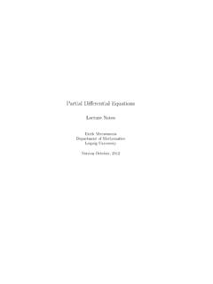
9 FILM CASTING. Today's society has in great abundance products that are made from polymers: clothing made from synthetic fibers, plastic bags, food wrap, and disposable diapers are among the most common examples. It has become imperative for today's manufacturers to understand the processes used to make these products as fully as possible. The processes involve complex fluid flow of a molten polymer, governed by systems of DEs. Film casting is an industrial process in which fluid (molten polymer) is extruded from a rectangular die of thickness e 0 and length l 0 , at a temperature T0 , and a velocity u 0 . Please see [1], [3], [6], [9] [12], and [13] for a detailed description of the process. The fluid is then stretched in the air due to the constant pulling force F of the chill roll, located at a distance of L.

10 From the die. The film is then cooled on this chill roll to solidify the fluid. The film casting process is shown in Figure 4. Figure 4: Schematic of the film casting process. 237. The five dependent variables of the flow are length l , velocity u , pulling force F , temperature T , and thickness e . Under certain assumptions, the equations governing this process may be 2 F 2. dl 12 u 2 36 u2 2 A l2. F. dx 2l A. du 1 F dF du 8 l2 Au A Ag A. dx 24 A dx dx dT 2 de d e dl e du e hT T T4 T4. dx C p ue dx dx dx l dx u given as follows. This is a system of five first order nonlinear ODEs. Further, while the initial conditions for length, velocity, temperature, and thickness are simply those at the die exit, the initial pulling force F0 is not known a priori.