Transcription of Pump Curves - 依耐水泵网
1 Fluid flow pump system Pump Types Fluid flow applications can be divided into two categories: low flow at high pressure and high flow at low pressure . Low flow at high pressure applications include hydraulic power systems and typically employ positive-displacement pumps . The vast majorities of fluid-flow applications are categorized as high flow at low pressure and typically use centrifugal pumps . The following analysis is for high flow at low pressure applications only. In centrifugal pumps , the fluid enters along the centerline of the pump, is pushed outward by the rotation of the impeller blades, and exits along the outside of the pump. A schematic of a centrifugal pump is shown below.
2 Centrifugal pump Pump Curves pumps can generate high volume flow rates when pumping against low pressure or low volume flow rates when pumping against high pressure. The possible combinations of total pressure and volume flow rate for a specific pump can be plotted to create a pump curve. The curve defines the range of possible operating conditions for the pump. If a pump is offered with multiple impellers with different diameters, manufacturers typically plot a separate pump curve for each size of impellor on the same pump performance chart. Smaller impellors produce less pressure at lower flow rates. Pump performance charts with multiple pump Curves are shown below. Typical pump performance charts.
3 Source: McQuiston and Parker, 1994, Heating Ventilating and Air Conditioning, John Wiley and Sons, Inc. The power required to push the fluid through the pipe, Wfluid, is the product of the volume flow rate and system pressure drop. Wfluid = V Ptotal Graphically, fluid work is represented by the area under the rectangle defined by the operating point on a pump performance chart. Typically, the efficiency of the pump at converting the power supplied to the pump into kinetic energy of the fluid is also plotted on the pump performance chart. Pump efficiencies typically range from about 50% to 80%. Power that is not converted into kinetic energy is lost as heat. The power required by the pump, which is sometimes called the shaft work or brake horsepower , can be calculated from the flow rate, total pressure, and efficiency values from the pump curve, using the following equation.
4 Wpump = Wfluid / Effpump = V Ptotal / Effpump A dimensional version of this equation, using units for pumping water at standard conditions, is: Wpump (hp) = V (gal/min) Ptotal (ft-H20) / (3,960 (gal-ft/min-hp) x Effpump) Many pump performance graphs, including those shown above, also plot Curves showing the work required by the pump to produce a specific flow and pressure. Note that these Curves show work required by the pump including the efficiency of the pump. Calculating the work supplied to the pump using the preceding equation and comparing it to the value indicated on a pump performance graph is a useful exercise. System Curve The total pressure that the pump must produce to move the fluid is determined by the piping system.
5 This total pressure of the piping system is the sum of the pressure due to inlet and outlet conditions and the pressure loss due to friction. In a piping system, pressure loss due to friction increases with increasing fluid flow; thus, system Curves have positive slopes on pump performance charts. The operating point of a pump is determined by the intersection of the pump and system Curves . To determine the form of a system curve, consider the equation for total pressure in a piping system. The total pressure caused by a piping system is the sum of the pressure due to inlet and outlet conditions and the pressure required to overcome friction through the pipes and fittings. Ptotal = ( Pstatic + Pvelocity + Pelevation )inlet-outlet + Pfricition Inlet/Outlet Pressure The inlet/outlet pressure that the pump must overcome is the sum of the static, velocity and elevation pressures between the inlet and outlet of the piping system.
6 For closed loop piping systems, the inlet and outlet are at the same location; hence, the static, velocity and elevation pressure differences are all zero. For open systems, the differences in static, velocity and elevation pressures must be calculated (See Fluid_Flow Piping). In many pumping applications, the velocity pressure difference between the inlet and outlet is zero or negligible, and inlet/outlet pressure is simply the sum of the static and elevation heads. In these cases, the inlet/outlet pressure is independent of flow and is represented on a pump performance chart as the pressure at zero flow. Friction Pressure Drop Friction between the fluid and pipe walls and fittings increases with the volume flow rate.
7 The equations for pressure loss from friction through the fittings, hlf, and pressure loss from friction with the pipes, hlp, show that in each case friction pressure drop is proportional to the square of velocity: hlf = kf V2 / 2 hlp = (f L V2) / (2 D) Velocity is proportional to volume flow rate; hence, friction pressure drop is also proportional to the square of volume flow rate. Pheadloss = (hl) = (hlf + hlp) = [ (kf V2 / 2) + ((f L V2) / (2 D)) ] = C1 V2 = C2 V2 This quadratic relationship can be plotted on the pump curve to show the friction component of the system curve . Plotting a System Curve As the preceding discussion showed, system Curves have a flow-independent component (of inlet/outlet pressure) and a flow-dependent component that varies with the square of flow rate (of friction pressure).
8 A system curve for a closed-loop piping system with no inlet/outlet pressure difference is shown below. The curve is a parabola of the form Pheadloss = C2 V2. The curve passes through the origin because the inlet/outlet pressure difference, sometimes called the static head, is zero. The coefficient C2 can be determined if the operating point is known by substituting the known pressure drop and flow rate into the equation and solving for C2. The fluid work required to push the fluid through the pipe is the product of the volume flow rate and system pressure drop and is represented graphically by the area under the rectangle defined by the operating point. Source of original pump curve: Kreider and Rabl, 1996.
9 A system curve for an open-loop piping system with a static or inlet/outlet pressure of 40 ft is shown below. This system curve is of the form P headloss = A + C2 V2; where A is the static or inlet/outlet pressure drop. As before, the coefficient C2 can be determined if the operating point and inlet/outlet pressure are known by substituting the known values into the equation and solving for C2. Source of original pump curve: Kreider and Rabl, 1996. Variation of Pump Efficiency With Impeller Diameter and Rotational Speed Pump efficiency is greatest when the largest possible impeller is installed in a pump casing. Pump efficiency decreases when smaller impellers are installed in a pump because of the increased amount of fluid that slips through the space between the tips of the impeller blades and the pump casing.
10 The pump performance charts shown above clearly show the decrease in pump efficiency with smaller impellers. Pump efficiency also decreases as the rotational speed of a pump is reduced. However, the magnitude of the decrease in pump efficiency depends on the individual pump. For example, in the pump performance chart shown below, pump efficiency declines from about 75% at full speed to about 55% at half speed while following the system curve with zero static head. For other pumps , the magnitude of the decrease in pump efficiency may be negligible. For example, in the pump performance chart shown below, pump efficiency at variable speeds remains constant for pumping systems following a system curve with zero static head, but decreases for pumping systems with high static head.