Transcription of Pump Station Design Guidelines Second Edition
1 Pump Station Design Guidelines Second Edition Jensen Engineered Systems 825 Steneri Way Sparks, NV 89431. For Design assistance call (855)468-5600. 2012 Jensen Precast TABLE OF CONTENTS. INTRODUCTION ..3. PURPOSE OF THIS GUIDE ..3. OVERVIEW OF A TYPICAL JES SUBMERSIBLE LIFT Station ..3. Design PROCESS ..3. BASIC PUMP SELECTION ..5. THE SYSTEM CURVE ..5. STATIC FRICTION LOSSES ..6. TOTAL DYNAMIC HEAD ..9. HOW pumps WORK ..13. OVERVIEW OF A SUBMERSIBLE BASIC IMPELLER THEORY ..14. THE CASING ..14. THE INLET ..14. IMPELLER TYPES ..15. MOTORS ..17. MECHANICAL SEALS ..19. PUMP CURVES ..22. STEEPNESS OF PUMP CURVE ..24. INTERACTION OF THE SYSTEM CURVE WITH THE PUMP CURVE ..24. NET POSITVE SUCTION HEAD ..25. INTRODUCTION TO WET WELL Design ..26. MINIMUM STORAGE VOLUME ..27. SIZE OF WELL ..28. HATCH SIZING ..28. DIAMETER OF WELL ..31. CONTROL ELEVATIONS ..32. HX MINIMUM SUBMERGENCE.
2 33. HMIN MINIMUM STORAGE ..34. HLAG LAG STORAGE ..34. HRES RESERVOIR STORAGE ..34. 2. INTRODUCTION. PURPOSE OF THIS GUIDE. The intent of this manual is to guide the engineering professional through a typical Design of a Jensen Engineered Systems (JES) packaged lift Station . These are the same steps and procedures followed by our engineers when we are designing a submersible lift Station . JES can always provide you with a project specific Design free of charge. Simply contact one of our Design professionals toll free at (855) 468-5600. For those who would like insight into our basis of Design , or want to be more hands on in the Design process, we hope this manual is of help. OVERVIEW OF A TYPICAL JES SUBMERSIBLE LIFT Station . Figure 1. A typical submersible lift Station by JES includes a wet well, dual submersible pumps , valves and an electronic pump control system. In smaller stations, the valves will often be installed in the wet well to save infrastructure costs.
3 On larger systems, it is recommended that a separate valve vault be specified to provide easy access in the event maintenance is necessary. Design PROCESS. The typical Design process starts with understanding what type of water needs to be pumped, and the volume of that water. Most JES submersible lift Station applications are intended for either stormwater or wastewater. This is an important step, not only because of the obvious differences between the fluids, but also because of some not- so obvious implications which will be discussed later. 3. Determining the volume of the fluid can be as simple as identifying the fixture unit count in a residential home, or as complicated as preparing a detailed hydrology report for a 50-acre commercial site. The intent of this manual is not to detail these very broad subjects, but to point out the necessity of properly determining flowrates, as well as provide a good understanding of the occurrence of those flows and how they relate to a pump Station .
4 Figure 2. The next steps in Design are site considerations. How far does the lift Station need to pump? How high does the liquid need to rise? These questions, when coupled with the flowrate, are eventually going to determine the size of pump the system will require. Additional site considerations, such as whether or not the lift Station is located in a roadway, will play into various other Design criteria. The better the understanding of the site, the easier the lift Station will be to Design . Once flow has been determined and site considerations have been taken into account, the system curve can be developed. The system curve is matched with various pump curves in an iterative process to determine which pump will best match the demands of the project. Once the pump is selected, all the additional components, such as the wet well, valve vault, valve and pipes, control system, etc.
5 , can be sized. 4. BASIC PUMP SELECTION. THE SYSTEM CURVE. The most important part of any pump selection is first determining the system curve. This means, at the very least, the flowrate and head that will be required of the pump must be identified. Often this is the first mistake made in the selection process. In many potable water booster stations, the flowrate is determined by a downstream demand. In a typical JES. application, the purpose of the lift Station is to simply move water from one location to another. Therefore, the flow is typically governed by the inflow to the Station , and not an outflow demand. Once the flowrate into the Station is found, the amount of head required by the pump can be determined by calculating the system losses in the piping network. Rule of thumb estimates and outright guesses of the friction losses will lead to poorly sized equipment that will have a poor efficiency and reliability.
6 Calculation of the system losses at several different flowrates will yield a system curve. System curves represent a loss of energy in systems with a variation in the flowrate. Or, stated differently, the amount of energy the pump must generate to operate at a given flowrate. System losses come in two forms that are outlined below. STATIC LOSSES. Static losses are due to differences in either elevation or pressure between the inlet and the discharge. In some booster pump systems, the discharge could be in a pressurized holding tank. So tank pressure must be taken into consideration during Design . In a typical JES lift Station , the force main discharges to gravity in either a manhole or other holding structure. Figure 3. In figure 3, the static head (in Feet) is the difference between the discharge elevation of the force main and the water level of the wet well. It is important to note the difference between condition A' and condition B'.
7 While the pumps are in the off position, the water level in the wet well rises. When the water level reaches a pre- determined storage elevation, the pumps turn on and the surface elevation draws down until it reaches the pumps 5. off position. Determining these elevations will be addressed later, but for now it is important to understand that the static head is not a fixed value, but rather a floating value dependent upon the water surface elevation in the wet well. Many designers consider the system curve to be a fixed and unchanging representation of the pumping system. However, because the system curve is based upon the static head, which is a fluctuating variable, the system curve itself can fluctuate. Therefore, the system curve is not a single point set It is a range of curves. This will become more apparent when developing a system curve is discussed later in this manual.
8 FRICTION LOSSES. The Second part of losses in the pumping system are the dynamic losses. Dynamic losses are dependent upon the flowrate through the system and primarily attributed to the system friction. This includes friction of the liquid flowing through the pipe and fittings, as well as the friction internal to the fluid itself. The friction begins at the level of the total static head and increases with flowrate. The subject of friction losses in a piping network is vast and complex. Example: in designing a water booster Station for a residential neighborhood, a detailed pipe analysis of the network, including its physical characteristics and flow demands, would be necessary. Rather than delve deeper is determining these losses in this manual, the following discussion assumes a very simple, single force main, gravity discharge lift Station . For projects requiring a more complicated distribution system, contact Jensen Engineered Systems.
9 We utilize advanced computer modeling software to detail the piping network. There are many different methods for determining friction losses in a pipe. These include The Darcy-Weisbach Equation, along with the Hazen Williams Equation. We will be using the Hazen Williams Equation because of its relative ease for a simple force main. There are some limitations to the Hazen Williams Equation which will be discussed. To explore this subject in further detail, or learn more about other methods, there are some very good current publications: Pumping Station Design (Revised Third Edition ) by Jones, Sanks, Tchobanoglous, and Bosserman, published by Butterworth-Heinemann, is thought by many to be the most in-depth resource for pump Station Design . Another publication worth reviewing is Hydrology and Hydraulic Systems ( Second Edition ) by Gupta, published by Waveland Press, Inc. There are some advantages of using the Hazen Williams Equation.
10 Not only is it simple and easy to use, its use is also required by many regulatory agencies. The Hazen Williams Equation is somewhat constraining because there must be turbulent flow within the pipe, and the fluid type must be water that is at, or near, room temperature. Additionally, the fluid velocity must be between 3 to 9 ft/sec. This last constraint actually lends itself quite well to wastewater lift Design because if the wastewater velocity is below 3 ft/sec., there will not be enough energy to scour the pipe of solids. Conversely, water flowing above 9 ft/sec. can scour the pipe material and damage the force main. The final constraint is that the Hazen-Williams Equation should not be used on force mains larger than 60 in diameter. 6. HAZEN WILLIAM EQUATION. The base form of the Hazen William Equation is as follows: Equation 1. v = velocity (ft/sec). C = Hazen Williams friction coefficient R = hydraulic radius (feet).