Transcription of Readers will be provided a link to download the software
1 Readers will be provided a link to download the software and Excel files that are used in the book after payment. Please visit for more information on the book. The Excel files are compatible with Excel 2003, 2007 and 2010. Chapter 1: Basic Forecasting Methods p/g 1 moving Average Forecast a country farm production Exponential Smoothing Forecast a country farm production Holts Method Forecast a winter clothing sales Holts Winters Forecast fishing rods sales Chapter 2: ARIMA / Box Jenkins p/g 24 Arima Modeling Subjective Method Example 1: Daily Sales Forecasting Objective Method Example 2: Forecast daily electricity production Chapter 3: Monte Carlo Simulation p/g 81 Example 1: Coin Tossing Example 2: Sales Forecasting Example 3: Modeling Stock Prices Chapter 4: K Nearest Neighbors p/g 103 Example 1: KNN for classification of home ownership Example 2: KNN for time series prediction with stock market data Example 3: Cross Validation With MSE Chapter 5: Neural Network With MS Excel p/g 117 Example 1: Credit Approval Model Example 2: Sales Forecasting Example 3.
2 Predicting Stock Prices (DJIA) Example 4: Predicting Real Estate Value Example 5: Classify Type Of Flowers Chapter 6: Markov Chain with MS Excel p/g 218 Example 1: Predict delivery time for a courier company Example 2: Predict brand loyalty of soft drink customers Chapter 7: Bayes Theorem with MS Excel p/g 231 Example 1: Predict rainy or sunny day Example 2: Predict stock market trend Appendix A p/g 239 How to use nn_Solve Appendix B p/g 241 Simple Linear Regression For Forecasting Appendix C p/g 251 How to access Excel Solver 2007 and 2010 1 Chapter 1: Basic Forecasting Methods Introduction Forecasting is the estimation of the value of a variable (or set of variables) at some future point in time. In this book we will consider some methods for forecasting. A forecasting exercise is usually carried out in order to provide an aid to decision-making and in planning the future.
3 Typically all such exercises work on the premise that if we can predict what the future will be like we can modify our behaviour now to be in a better position, than we otherwise would have been, when the future arrives. Applications for forecasting include: inventory control/production planning - forecasting the demand for a product enables us to control the stock of raw materials and finished goods, plan the production schedule, etc investment policy - forecasting financial information such as interest rates, exchange rates, share prices, the price of gold, etc. This is an area in which no one has yet developed a reliable (consistently accurate) forecasting technique (or at least if they have they haven't told anybody!) economic policy - forecasting economic information such as the growth in the economy, unemployment, the inflation rate, etc is vital both to government and business in planning for the future.
4 Types of forecasting problems/methods One way of classifying forecasting problems is to consider the timescale involved in the forecast how far forward into the future we are trying to forecast. Short, medium and long-term are the usual categories but the actual meaning of each will vary according to the situation that is being studied, in forecasting energy demand in order to construct power stations 5-10 years would be short-term and 50 years would be long-term, whilst in forecasting consumer demand in many business situations up to 6 months would be short- term and over a couple of years long-term. The table below shows the timescale associated with business decisions. 2 Timescale Type of decision Examples Short-term up to 3-6 months Operating Inventory control, Production planning, distribution Medium-term up to 3-6 moths to 2 years months Tactical Leasing of plant and equipment, Employment changes Long-term above 2 years Strategic Research and development Acquisitions and mergers, Product changes The basic reason for the above classification is that different forecasting methods apply in each situation, a forecasting method that is appropriate for forecasting sales next month (a short-term forecast) would probably be an inappropriate method for forecasting sales in five years time (a long-term forecast).
5 In particular note here that the use of numbers (data) to which quantitative techniques are applied typically varies from very high for short-term forecasting to very low for long-term forecasting when we are dealing with business situations. Some areas can encompass short, medium and long term forecasting like stock market and weather forecasting. Forecasting methods can also be classified into several different categories: qualitative methods - where there is no formal mathematical model, often because the data available is not thought to be representative of the future (long-term forecasting) quantitative methods - where historical data on variables of interest are available these methods are based on an analysis of historical data concerning the time series of the specific variable of interest and possibly other related time series and also examines the cause-and-effect relationships of the variable with other relevant variables time series methods - where we have a single variable that changes with time and whose future values are related in some way to its past values.
6 This chapter will give a brief overview of some of the more widely used techniques in the rich and rapidly growing field of time series modeling and analysis. We will deal with qualitative and quantitative forecasting methods on later chapters. Areas covered in this Chapter are: a) Simple moving Average b) Weighted moving Average c) Single Exponential Smoothing d) Double Exponential Smoothing (Holt s Method) 3 e) Triple Exponential Smoothing (Holt Winters Method) These methods are generally used to forecast time series. A time series is a series of observations collected over evenly spaced intervals of some quantity of interest. number of phone calls per hour, number of cars per day, number of students per semester, daily stock Let yi = observed value i of a time series (i = 1,2,..,t) yhati = forecasted value of yi ei = error for case i = yi yhati Sometimes the forecast is too high (negative error) and sometimes it is too low (positive error).
7 The accuracy of the forecasting method is measured by the forecasting errors. There are two popular methods for assessing forecasting accuracy: Mean Absolute Deviation (MAD) MAD = ( | ei | )/n => sum of errors divided by the number of periods in the forecast Where n is the number of periods in the forecast; ei = error Units of MAD are same as units of yi Mean Squared Error (MSE) MSE = ( ei 2 )/n => sum of squared errors divided by the number of periods in the forecast a) Single moving Average This simplest forecasting method is the moving average forecast. The method simply averages of the last n observations. It is useful for time series with a slowly changing mean. Use an average of the N most recent observations to forecast the next period. From one period to the next, the average moves by replacing the oldest observation in the average with the most recent observation.
8 In the process, short-term irregularities in the data series are smoothed out . The general expression for the moving average is 4 yhati = [ yt + yt-1 + .. + yt-N+1] / N How do you choose N? We want the value of N that gives us the best forecasting accuracy. ( minimizes MAD or MSE). Let s look at an example. Open workbook TimeSeries in the folder Chapter 1 and goto to Worksheet (Milk Data). Here we have the daily record of milk production of a country farm. Figure Next, goto Worksheet (ma solution).We will use N = 3, so we enter the formula =AVERAGE(B6:B8) in cell C9. This formula is simply [ yt + yt-1 + yt-2] / 3. (see Fig below) 5 Figure After that we fill down the formula until C25. We take the absolute error at column D and squared error at column E. See all the formula enter in Fig below.
9 We have the MAD = in cell D27 and MSE = in cell E27. If at day 20 we have 49 gallons, how do you forecast the production at day 21? To forecast simply fill down the formula in cell C25 to cell C26 or enter the formula =AVERAGE(B23:B25). Here the result is gallons. (see Figure ) As you can see with this example, the moving average method is very simple to build. You can also experiment with N = 4 or to see whether you can get a lower MAD and MSE 6 Figure b) Weighted moving Average In the moving averages method above, each observation in the average is equally weighted whereas the weighted moving averages method, typically the most recent observation carries the most weight in the average. The general expression for weighted moving average is yhati = [ wt*yt + wt-1*yt-1 + .. + wt-N+1* yt-N+1] Let wi = weight for observation i wt = 1 => The sum of the weights is 1.
10 To illustrate, let s rework the milk example. Goto Worksheet (wma solution). Using a weight of .5 enter in cell H2 for the most recent observation, a weight of .3 in cell H3 for the next most recent observation, and a weight of .2 in cell H4 for the oldest observation. (see Figure ) Again using N =3, we enter the formula =(B8*$H$2+B7*$H$3+B6*$H$4) in cell C9 and fill down to C25. (Note: we use the $ sign to lock the cell in H2, H3 and H4). 7 Figure The absolute error and squared error are entered in column D and E respectively. Cell D27 show the MAD and cell E27 is the MSE. Could we have used a better set of weights than those above in order to have a better forecast? Let use Excel Solver to check for you. Choose Tools, Solver from the menu. (See Appendix C on how to access Excel 2007 and Excel 2010 Solver) Figure Upon invoking Solver from the Tools menu, a dialogue box appears as in Fig below 8 Figure Next we will enter all the parameters in this dialogue box.