Transcription of rfm clv 2005-02-16 - Bruce Hardie's Home Page
1 RFM and CLV: Using Iso-value Curvesfor Customer Base AnalysisPeter S. FaderBruce G. S. HardieKa Lok Lee1 July 2004 Revised December 2004 Revised February 20051 Peter S. Fader is the Frances and Pei-Yuan Chia Professor of Marketing at the Wharton School of theUniversity of Pennsylvania (address: 749 Huntsman Hall, 3730 Walnut Street, Philadelphia, PA 19104-6340; phone: ; ). Bruce G. is Associate Professor of Marketing, London Business School Ka Lok Lee is Market Research Analyst, Catalina Health Resource The authors thank Albert Bemmaor, Paul Farris, Phil Pfeifer, threeanonymous referees, and seminar participants at the Yale SOM and University of Auckland for theirhelpful comments. The second author acknowledges the support of the London Business School Centrefor and CLV: Using Iso-value Curves for Customer Base AnalysisWe present a new model that links the well-known RFM (recency, frequency, monetary value)paradigm with customer lifetime value (CLV).
2 While previous researchers have connected thetwo conceptually, none has presented a formal model that requires nothing more than RFMinputs to make specific lifetime value projections for a set of customers. Key to this analysis isthe notion of iso-value curves, which enable us to group together individual customers whohave different behavioral histories but similar future valuations. Iso-value curves make it easy tovisualize and summarize the main interactions and tradeoffs among the RFM measures and stochastic model, featuring a Pareto/NBD framework to capture the flow of transactionsover time and a gamma-gamma sub-model for dollars per transaction, reveals a number of subtlebut important non-linear associations that would be missed by relying on observed data conduct a number of holdout tests to demonstrate the validity of the model s underlyingcomponents, and then focus on our iso-value analysis to estimate the net present value for a largegroup of customers of the online music site, CDNOW.
3 We summarize a number of substantiveinsights and point out a set of broader issues and opportunities in applying such a model inactual :customer lifetime value, CLV, RFM, customer base analysis, Pareto/NBD1 IntroductionThe move towards a customer-centric approach to marketing, coupled with the increasing avail-ability of customer transaction data, has led to an interest in both the notion and calculationof customer lifetime value (CLV).At a purely conceptual level, the calculation of CLV is a straightforward proposition: it issimply the present value of the future cashflows associated with a customer (Pfeifer et al. 2005 ).Because of the challenges associated with forecasting future revenue streams, most empiricalresearch on lifetime value has actually computed customer profitability based solely on cus-tomers past behavior. But in order to be true to the notion of CLV, our measures should lookto the future, not the past.
4 A significant barrier has been our ability to model future revenuesappropriately, particularly in the case of a noncontractual setting ( , where the time atwhich customers become inactive is unobserved) (Bell et al. 2002, Mulhern 1999).A number of researchers and consultants have developed scoring models ( , regression-type models) that attempt to predict a customer s future behavior. (See, for example, Baesens etal. (2002), Berry and Linoff (2004), Bolton (1998), Malthouse (2003), Malthouse and Blattberg( 2005 ), Parr Rud (2001).) In examining this work, we note that measures of a customer spast behavior are key predictors of their future behavior. Drawing on the direct marketingliterature, it is common practice to summarize a customer s past behavior in terms of their RFM characteristics:recency(time of most recent purchase),frequency(number of pastpurchases), andmonetary value(average purchase amount per transaction).
5 But there are several problems with these models, especially when seeking to develop CLVestimates: Scoring models attempt to predict behavior in the next period. But when computing CLV,we are interested not only in period 2; we also need to predict behavior in periods 3, 4, 5,and so on. It is not clear how a regression-type model can be used to forecast the dynamicsof buyer behavior well into the future and then tie it all back into a present value foreach customer. Two periods of purchasing behavior are required period 1 to define the RFM variables1and period 2 to arrive at values of the dependent variable(s). It would be better if wewere able to create predictions of future purchasing behavior simply using period 1 dataalone. More generally, it would be nice to be able to leverage all of the available data formodel calibration purposes without using any of it to create a dependent variable for aregression-type analysis.
6 The developers of these models ignore the fact that the observed RFM variables areonly imperfect indicators of underlying behavioral traits (Morrison and Silva-Risso 1995).1 They fail to recognize that different slices of the data will yield different values of theRFM variables and therefore different scoring model parameters. This has important im-plications when we utilize the observed data from one period to make predictions of way to overcome these general problems is to develop a formal model of buyer behavior,rooted in well-established stochastic models of buyer behavior. In developing a model based onthe premise that observed behavior is a realization of latent traits, we can use Bayes theorem toestimate an individual s latent traits as a function of observed behavior and then predict futurebehavior as a function of these latent traits. At the heart of our model is the Pareto/NBDframework (Schmittlein, Morrison, and Colombo 1987) for the flow of transactions over time ina noncontractual setting.
7 An important characteristic of our model is that measures of recency,frequency, and monetary value are sufficient statistics for an individual customer s purchasinghistory. That is, rather than including RFM variables in a scoring model simply because of theirpredictive performance as explanatory variables, we formally link the observed measures to thelatent traits and show that no other information about customer behavior is required in orderto implement our conveying our analytical results, we offer a brief exploratory analysis to set the stagefor our model development. Let us consider the purchasing of the cohort of 23,570 individualswho made their first-ever purchase at CDNOW in the first quarter of 1997. We have datacovering their initial and subsequent ( , repeat) purchases up to the end of June 1998. (See1 This same problem besets Dwyer s customer migration model (Berger and Nasr 1998, Dwyer 1989) and itsextensions (Pfeifer and Carraway2000).)
8 2 Fader and Hardie 2001 for further details about this dataset.) For presentational simplicity,we initially examine the relationship between future purchasing and recency/frequency alone;we will introduce monetary value later in the paper. We first split the 78-week dataset intotwo periods of equal length, and group customers on the basis of frequency (wherexdenotesthe number of repeat purchases in the first 39-week period) and recency (wheretxdenotes thetime of the last of these purchases). We then compute the average total spend for each of thesegroups in the following 39-week data are presented in Figure +$0$100$200$300$400 Recency (tx)Frequency (x)Avg. Total Spend in Wks 40 78 Figure 1: Average Total Spend in Weeks 40 78 by Recency and Frequency in Weeks 1 39It is clear that recency and frequency each has a direct and positive association with futurepurchasing, and there may be some additional synergies when both measures are high ( , inthe back corner of the figure).
9 But despite the large number of customers used to generate thisgraph, it is still very sparse and therefore somewhat untrustworthy. A number of the valleys in Figure 1 are simply due to the absence of any observations for particular combinations ofrecency and frequency. It is important for us to abstractawayfrom the observed data anddevelop a formal model in order to fill in the blanks. An alternative view of the same relationship is shown in Figure 2. This contour plot, or 30,000 ft view of Figure 1, is an example of an iso-value plot; each curve in the graphlinks together customers with equivalent future value despite differences in their past have removed the purchasing data for ten buyers who purchased over $4000 worth of CDs across the78-week period. According to our contacts at CDNOW, these people are probably unauthorized resellers whoshould not be analyzed in conjunction with ordinary customers.
10 This initial exploratory analysis is thereforebased on the purchasing of 23,560 , it is easy to see how higher recency and higher frequency are correlated with greaterfuture purchasing, but the jagged nature of these curves highlights the dangers of relying solelyon observed data in the absence of a +Recency (tx)Frequency (x)5050505050505050505050505050505050505 0505050100100100100100100100100100100100 100100100100100100200200200200200300300 Figure 2: Contour Plot of Average Week 40 78 Total Spend by Recency and FrequencyWe should also note that in using such plots to understand the nature of the relationshipbetween future purchasing and recency/frequency, the patterns observed will depend on theamount of time for which the customers are observed ( , the length of periods 1 and 2).But despite these limitations in attempting to use the kind of data summaries shown inFigures 1 and 2, there is still clear diagnostic value in the general concept of iso-value curvesfor customer base analysis.