Transcription of Rootfinding for Nonlinear Equations
1 > 3. Rootfinding Rootfinding for Nonlinear Equations 3. Rootfinding Math 1070. > 3. Rootfinding Calculating the roots of an equation f (x) = 0 ( ). is a common problem in applied mathematics. We will explore some simple numerical methods for solving this equation, and also will consider some possible difficulties 3. Rootfinding Math 1070. > 3. Rootfinding The function f (x) of the equation ( ). will usually have at least one continuous derivative, and often we will have some estimate of the root that is being sought. By using this information, most numerical methods for ( ) compute a sequence of increasingly accurate estimates of the root.
2 These methods are called iteration methods. We will study three different methods 1 the bisection method 2 Newton's method 3 secant method and give a general theory for one-point iteration methods. 3. Rootfinding Math 1070. > 3. Rootfinding > The bisection method In this chapter we assume that f : R R , f (x) is a function that is real valued and that x is a real variable. Suppose that f (x) is continuous on an interval [a, b], and f (a)f (b) < 0 ( ). Then f (x) changes sign on [a, b], and f (x) = 0 has at least one root on the interval.
3 Definition The simplest numerical procedure for finding a root is to repeatedly halve the interval [a, b], keeping the half for which f (x) changes sign. This procedure is called the bisection method, and is guaranteed to converge to a root, denoted here by . 3. Rootfinding Math 1070. > 3. Rootfinding > The bisection method Suppose that we are given an interval [a, b] satisfying ( ) and an error tolerance > 0. The bisection method consists of the following steps: a+b B1 Define c = 2 . B2 If b c , then accept c as the root and stop.
4 B3 If sign[f (b)] sign[f (c)] 0, then set a = c. Otherwise, set b = c. Return to step B1. The interval [a, b] is halved with each loop through steps B1 to B3. The test B2 will be satisfied eventually, and with it the condition | c| . will be satisfied. Notice that in the step B3 we test the sign of sign[f (b)] sign[f (c)] in order to avoid the possibility of underflow or overflow in the multiplication of f (b). and f (c). 3. Rootfinding Math 1070. > 3. Rootfinding > The bisection method Example Find the largest root of f (x) x6 x 1 = 0 ( ).
5 Accurate to within = With a graph, it is easy to check that 1 < < 2. We choose a = 1, b = 2; then f (a) = 1, f (b) = 61, and ( ) is satisfied. 3. Rootfinding Math 1070. > 3. Rootfinding > The bisection method Use The results of the algorithm B1 to B3: n a b c b c f (c). 1 2 3 4 5 6 7 8 9 10 Table: Bisection Method for ( ). The entry n indicates that the associated row corresponds to iteration number n of steps B1 to B3. 3. Rootfinding Math 1070. > 3. Rootfinding > Error bounds Let an , bn and cn denote the nth computed values of a, b and c: 1.
6 Bn+1 an+1 = (bn an ), n 1. 2. and 1. bn an = (b a) ( ). 2n 1. where b a denotes the length of the original interval with which we started. Since the root [an , cn ] or [cn , bn ], we know that 1. | cn | cn an = bn cn = (bn an ) ( ). 2. This is the error bound for cn that is used in step B2. Combining it with ( ), we obtain the further bound 1. | cn | (b a). 2n This shows that the iterates cn as n . 3. Rootfinding Math 1070. > 3. Rootfinding > Error bounds To see how many iterations will be necessary, suppose we want to have | cn |.
7 This will be satisfied if 1. (b a) . 2n Taking logarithms of both sides, we can solve this to give log b a .. n . log 2. For the previous example ( ), this results in 1.. log . n = log 2. , we need n = 10 iterates, exactly the number computed. 3. Rootfinding Math 1070. > 3. Rootfinding > Error bounds There are several advantages to the bisection method It is guaranteed to converge. The error bound ( ) is guaranteed to decrease by one-half with each iteration Many other numerical methods have variable rates of decrease for the error, and these may be worse than the bisection method for some Equations .
8 The principal disadvantage of the bisection method is that generally converges more slowly than most other methods. For functions f (x) that have a continuous derivative, other methods are usually faster. These methods may not always converge; when they do converge, however, they are almost always much faster than the bisection method. 3. Rootfinding Math 1070. > 3. Rootfinding > Newton's method Figure: The schematic for Newton's method 3. Rootfinding Math 1070. > 3. Rootfinding > Newton's method There is usually an estimate of the root , denoted x0.
9 To improve it, consider the tangent to the graph at the point (x0 , f (x0 )). If x0 is near , then the tangent line the graph of y = f (x) for points about . Then the root of the tangent line should nearly equal , denoted x1 . 3. Rootfinding Math 1070. > 3. Rootfinding > Newton's method The line tangent to the graph of y = f (x) at (x0 , f (x0 )) is the graph of the linear Taylor polynomial: p1 (x) = f (x0 ) + f 0 (x0 )(x x0 ). The root of p1 (x) is x1 : f (x0 ) + f 0 (x0 )(x1 x0 ) = 0. , f (x0 ). x1 = x0 . f 0 (x0 ). 3. Rootfinding Math 1070.
10 > 3. Rootfinding > Newton's method Since x1 is expected to be an improvement over x0 as an estimate of , we repeat the procedure with x1 as initial guess: f (x1 ). x2 = x1 . f 0 (x1 ). Repeating this process, we obtain a sequence of numbers, iterates, x1 , x2 , x3 , .. hopefully approaching the root . The iteration formula f (xn ). xn+1 = xn , n = 0, 1, 2, .. ( ). f 0 (xn ). is referred to as the Newton's method, or Newton-Raphson, for solving f (x) = 0. 3. Rootfinding Math 1070. > 3. Rootfinding > Newton's method Example Using Newton's method, solve ( ) used earlier for the bisection method.