Second-Order Linear Differential Equations - …

1 Second-Order Linear Differential EquationsA Second-Order Linear Differential equationhas the formwhere ,, , and are continuous functions. We saw in Section that Equations ofthis type arise in the study of the motion of a spring. In Additional Topics: Applications ofSecond- order Differential Equationswe will further pursue this application as well as theapplication to electric this section we study the case where , for all , in Equation 1. Such equa-tions are called homogeneouslinear Equations . Thus, the form of a Second-Order linearhomogeneous Differential equation isIf for some , Equation 1 is nonhomogeneousand is discussed in AdditionalTopics: Nonhomogeneous Linear basic facts enable us to solve homogeneous Linear Equations . The first of these saysthat if we know two solutions and of such an equation, then the Linear combinationis also a and are both solutions of the Linear homogeneous equa-tion (2) and and are any constants, then the functionis also a solution of Equation and are solutions of Equation 2, we haveandTherefore, using the basic rules for differentiation, we haveThus,is a solution of Equation other fact we need is given by the following theorem, which is proved in moreadvanced courses.

2 It says that the general solution is a Linear combination of two linearlyindependentsolutions and This means that neither nor is a constant multipleof the other. For instance, the functions and are linearly dependent,but and are linearly x xexf x ext x 5x2f x c1y1 c2y2 c1 0 c2 0 0 c1 P x y1 Q x y1 R x y1 c2 P x y2 Q x y2 R x y2 P x c1y1 c2y2 Q x c1y1 c2y2 R x c1y1 c2y2 P x c1y1 c2y2 Q x c1y1 c2y2 R x c1y1 c2y2 P x y Q x y R x y P x y2 Q x y2 R x y2 0 P x y1 Q x y1 R x y1 0y2y1y x c1y1 x c2y2 x c2c1y2 x y1 x 3y c1y1 c2y2y2y1xG x 0P x d2ydx2 Q x dydx R x y 02xG x 0 GRQPP x d2ydx2 Q x dydx R x y G x 11 TheoremIf and are linearly independent solutions of Equation 2, and is never 0, then the general solution is given bywhere and are arbitrary 4 is very useful because it says that if we know twoparticular linearly inde-pendent solutions, then we know general, it is not easy to discover particular solutions to a Second-Order Linear equa-tion.

3 But it is always possible to do so if the coefficient functions , , and are constantfunctions, that is, if the Differential equation has the formwhere , , and are constants and .It s not hard to think of some likely candidates for particular solutions of Equation 5 ifwe state the equation verbally. We are looking for a function such that a constant timesits second derivative plus another constant times plus a third constant times is equalto 0. We know that the exponential function (where is a constant) has the prop-erty that its derivative is a constant multiple of itself:. Furthermore,.If we substitute these expressions into Equation 5, we see that is a solution iforBut is never 0. Thus,is a solution of Equation 5 if is a root of the equationEquation 6 is called the auxiliary equation(or characteristic equation) of the differen-tial equation . Notice that it is an algebraic equation that is obtainedfrom the Differential equation by replacing by ,by , and by.

4 Sometimes the roots and of the auxiliary equation can be found by factoring. Inother cases they are found by using the quadratic formula:We distinguish three cases according to the sign of the discriminant .CASE I In this case the roots and of the auxiliary equation are real and distinct, so and are two linearly independent solutions of Equation 5. (Note that is not aconstant multiple of .) Therefore, by Theorem 4, we have the following the roots and of the auxiliary equation are real andunequal, then the general solution of isy c1er1x c2er2xay by cy 0ar2 br c 0r2r18er1xer2xy2 er2xy1 er1xr2r1b2 4ac 0b2 4acr2 b sb2 4ac2ar1 b sb2 4ac2a7r2r11yry r2y ay by cy 0ar2 br c 06ry erxerx ar2 br c erx 0 ar2erx brerx cerx 0y erxy r2erxy rerxry erxyy y ya 0cbaay by cy 05 RQPc2c1y x c1y1 x c2y2 x P x y2y142 Second-Order Linear Differential Equations 3 EXAMPLE 1 Solve the equation .SOLUTIONThe auxiliary equation iswhose roots are ,. Therefore, by (8) the general solution of the given differen-tial equation isWe could verify that this is indeed a solution by differentiating and substituting into thedifferential 2 Solve.

5 SOLUTIONTo solve the auxiliary equation we use the quadratic formula:Since the roots are real and distinct, the general solution isCASE II In this case ; that is, the roots of the auxiliary equation are real and equal. Let sdenote by the common value of and Then, from Equations 7, we haveWe know that is one solution of Equation 5. We now verify that is alsoa solution:The first term is 0 by Equations 9; the second term is 0 because is a root of the auxiliaryequation. Since and are linearly independent solutions, Theorem 4 pro-vides us with the general the auxiliary equation has only one real root , then thegeneral solution of isEXAMPLE 3 Solve the equation .SOLUTIONThe auxiliary equation can be factored as 2r 3 2 04r2 12r 9 04y 12y 9y 0y c1erx c2xerxay by cy 0rar2 br c 010y2 xerxy1 erxr 0 erx 0 xerx 0 2ar b erx ar2 br c xerx ay2 by2 cy2 a 2rerx r2xerx b erx rxerx cxerxy2 xerxy1 erx2ar b 0sor r2b2 4ac 0y c1e( 1 s13)x 6 c2e( 1 s13)x 6r 1 s1363r2 r 1 03 d2ydx2 dydx y 0y c1e2x c2e 3x 3r 2r2 r 6 r 2 r 3 0y y 6y 08_5_115f+gf+5gfgf-gg-ff+gFIGURE 1 In Figure 1 the graphs of the basic solutionsand of the differentialequation in Example 1 are shown in black andred, respectively.

6 Some of the other solutions, Linear combinations of and , are shown in x e 3xf x e2xSECOND- order Linear Differential EQUATIONS4 so the only root is . By (10) the general solution isCASE III In this case the roots and of the auxiliary equation are complex numbers. (See Appen-dix I for information about complex numbers.) We can writewhere and are real numbers. [In fact,,.] Then,using Euler s equationfrom Appendix I, we write the solution of the Differential equation aswhere ,. This gives all solutions (real or complex) of the dif-ferential equation. The solutions are real when the constants and are real. We sum-marize the discussion as the roots of the auxiliary equation are the complex num-bers ,, then the general solution of isEXAMPLE 4 Solve the equation .SOLUTIONThe auxiliary equation is . By the quadratic formula, theroots areBy (11) the general solution of the Differential equation isInitial-Value and Boundary-Value ProblemsAn initial-value problemfor the Second-Order Equation 1 or 2 consists of finding a solu-tion of the Differential equation that also satisfies initial conditions of the formwhere and are given constants.

7 If ,, , and are continuous on an interval andthere, then a theorem found in more advanced books guarantees the existenceand uniqueness of a solution to this initial-value problem. Examples 5 and 6 illustrate thetechnique for solving such a x 0 GRQPy1y0y x0 y1y x0 y0yy e3x c1cos 2x c2sin 2x r 6 s36 522 6 s 162 3 2ir2 6r 13 0y 6y 13y 0y e x c1cos x c2sin x ay by cy 0r2 i r1 i ar2 br c 011c2c1c2 i C1 C2 c1 C1 C2 e x c1cos x c2sin x e x C1 C2 cos x i C1 C2 sin x C1e x cos x isin x C2e x cos x isin x y C1er1x C2er2x C1e i x C2e i xei cos isin s4ac b2 2a b 2a r2 i r1 i r2r1b2 4ac 0y c1e 3x 2 c2xe 3x 2r 32 Figure 2 shows the basic solutionsand in Example 3 and some other members of the family of solutions. Notice that all of themapproach 0 as .xl t x xe 3x 2f x e 3x 2 FIGURE 28_5_225f+gf+5gfgf-gg-ff+g Figure 3 shows the graphs of the solu-tions in Example 4, and, together with some linearcombinations.

8 All solutions approach 0 as .xl t x e3x sin 2xf x e3x cos 2xFIGURE 33_3_32fgf-gf+gSECOND- order Linear Differential Equations 5 EXAMPLE 5 Solve the initial-value problemSOLUTIONFrom Example 1 we know that the general solution of the Differential equa-tion isDifferentiating this solution, we getTo satisfy the initial conditions we require thatFrom (13) we have and so (12) givesThus, the required solution of the initial-value problem isEXAMPLE 6 Solve the initial-value problemSOLUTIONThe auxiliary equation is , or , whose roots are . Thus,,and since , the general solution isSincethe initial conditions becomeTherefore, the solution of the initial-value problem isA boundary-value problemfor Equation 1 consists of finding a solution yof the dif-ferential equation that also satisfies boundary conditions of the formIn contrast with the situation for initial-value problems, a boundary-value problem doesnot always have a 7 Solve the boundary-value problemSOLUTIONThe auxiliary equation is r 1 2 0orr2 2r 1 0y 1 3y 0 1y 2y y 0y x1 y1y x0 y0y x 2cos x 3sin xy 0 c2 3y 0 c1 2 y x c1sin x c2cos x y x c1cos x c2sin xe0x 1 1 0 ir2 1r2 1 0y 0 3y 0 2y y 0y 35e2x 25e 3xc2 25 c1 35c1 23c1 1c2 23c1 y 0 2c1 3c2 013 y 0 c1 c2 112y x 2c1e2x 3c2e 3xy x c1e2x c2e 3xy 0 0y 0 1y y 6y 0 Figure 4 shows the graph of the solution ofthe initial-value problem in Example 5.

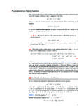
9 Comparewith Figure 4200_22 The solution to Example 6 is graphed in Figure 5. It appears to be a shifted sine curveand, indeed, you can verify that another way ofwriting the solution iswhere tan 23y s13sin x FIGURE 55_5_2 2 Second-Order Linear Differential EQUATIONS6 whose only root is . Therefore, the general solution isThe boundary conditions are satisfied ifThe first condition gives , so the second condition becomesSolving this equation for by first multiplying through by , we getsoThus, the solution of the boundary-value problem isSummary: Solutions of ay by c 0y e x 3e 1 xe xc2 3e 11 c2 3eec2e 1 c2e 1 3c1 1 y 1 c1e 1 c2e 1 3 y 0 c1 1y x c1e x c2xe xr 1 Roots ofGeneral solutiony e x c1 cos x c2 sin x r1, r2 complex: i y c1erx c2xerxr1 r2 ry c1er1x c2er2xr1, r2 real and distinctar2 br c 0 Figure 6 shows the graph of the solution ofthe boundary-value problem in Example 65_5_15 Exercises1 13 Solve the Differential ;14 16 Graph the two basic solutions of the Differential equationand several other solutions.

10 What features do the solutions have incommon? d2ydx2 2 dydx 5y 0d2ydx2 8 dydx 16y 06 d2ydx2 dydx 2y 0d2ydt2 dydt y 0d2ydt2 6 dydt 4y 0d2ydt2 2 dydt y 09y 4y 04y y 016y 24y 9y 04y y 03y 5y y 2y y 02y y y 0y 8y 41y 0y 4y 8y 0y 6y 8y 017 24 Solve the initial-value ,,18.,,19.,,20.,,21.,,22.,,23.,,24.,, 25 32 Solve the boundary-value problem, if ,,26.,,27.,,28.,,29.,,30.,,31.,,y 2 1y 0 2y 4y 13y 0y 1 0y 0 1y 6y 9y 0y 2y 0 1y 6y 25y 0y 5y 0 2y 100y 0y 3 0y 0 1y 3y 2y 0y 1 2y 0 1y 2y 0y 4y 0 34y y 0y 1 1y 1 0y 12y 36y 0y 0 1y 0 2y 2y 2y 0y 2y 0y 2y 5y 0y 4 4y 4 3y 16y 0y 0 4y 0 12y 5y 3y 0y 0 0 14y 4y y 0y 0 3y 0 1y 3y 0y 0 4y 0 32y 5y 3y 0 Click here for here for Linear Differential Equations 732.,, be a nonzero real number.(a)Show that the boundary-value problem ,,has only the trivial solution forthe cases and . 0 0y 0y L 0y 0 0y y 0Ly 1y 0 09y 18y 10y 0(b) For the case, find the values offor which this prob-lem has a nontrivial solution and give the , , and are all positive constants and is a solution of the Differential equation , show y x 0ay by cy 0y x cba 0 Second-Order Linear Differential EQUATIONS8 solutions approach 0 as and approach as.