Transcription of Second Welfare Theorem - University of Pittsburgh
1 Second Welfare TheoremEcon 2100 Fall 2018 Lecture 18, October 31 (boo)Outline1 Second Welfare TheoremFrom Last ClassWe want to state a prove a Theorem that says that any Pareto optimalallocation is (part of) a competitive will entail nding the prices that make that allocation an , we had to change the de nition of equilibrium to deal with an economy fXi;%i; !igIi=1;fYjgJj=1 , an allocationx ;y and a pricevectorp are a price equilibrium with transfers if there exists a vector ofwealth levelsw2 RLwithIXi=1wi=p IXi=1!i+JXj=1p y jsuch that:1. For eachj=1; :::;J:p yj p y jfor allyj2Yj;2.
2 For eachi=1; :::;I:x i%ixifor allxi2fxi2Xi:p xi wig; i IPi=1!i+JPj=1y j,withpl=0 if the inequlity is strict for x the boundary issues, we make another small nitionGiven an economyfXi;%igIi=1;fYjgJj=1; !, an allocationx ;y and a price vectorp constitute a quasi-equilibrium with transfers if there exists a vector of wealthlevelsw= (w1;w2; :::;wI)withIXi=1wi=p !+JXj=1p y jsuch that:1 For eachj=1; :::;J:p yj p y jfor everyi=1; :::;I:ifx ix ithenp x wi3 IPi=1x i IPi=1!i+JPj=1y jwithpl=0 if the inequlity is strict for sure you see why this deals with the previous equilibrium with transfers is a quasi-equilibrium (why?)
3 The maximzing condition for consumers is Welfare Theorem : PreliminariesWe have seen a few counterexamples to a possible Second Welfare Theorem ,and ways in which we can deal with is a summary of what we have learned so show that for any Pareto optimal allocation one can nd prices thatmake it into a competitive equilibrium requires a few assumptionsWe need transfers to overcome the limitations imposed by private need convexity of production need convexity and local non-satiation of need to eliminate boundary Welfare TheoremTheorem ( Second Fundamental Theorem of Welfare Economics)
4 Consider an economy fXi;%igIi=1;fYjgJj=1; ! and assume that Yjis convex forall j=1; :::;J, and%iis convex and locally non-satiated for all i=1; :::; , for each Pareto optimal allocation^x;^y there exists a price vector^p6=0suchthat(^x;^y;^p)form a quasi-equilibrium with proof uses the separating hyperplane an allocation is Pareto optimal there is an hyperplane that simultaneouslysupports the better-than sets of all consumers and all hyperplane yields a candidate equilibrium price proof is in three parts: aggregation, separation, and start with a Pareto optimal allocation and construct the correspondingquasi-equilibrium with of the Second Welfare Theorem .
5 AggregationFirst, we aggregate all consumers preferences when evaluating the Paretoe cient consumption bundle^ ne the following sets:Vi=fxi2Xi:xi ^xig RLandV=XiViVis the set of all bundles strictly preferred to^xby every : V is x0,x002Vi(so both are strictly preferred to^xi) and assumex0% preferences are convex, for any 2[0;1] x0+ (1 )x00%ix00By transitivity, we have x0+ (1 )x00%ix00 i^xiTherefore, x0+ (1 )x00is an element of Viand therefore each Viis is convex because it is the sum of I convex of the Second Welfare Theorem : AggregationSecond, we aggregate all rms and de ne the set of attainable ne the aggregate production set asY=XjYj=8<:Xjyj2RL:y12Y1; :::;yJ2YJ9=;The set of consumption bundles that can be allocated to consumers isY+f!
6 GThis set is convex since it is the sum ofJ+1 convex of the ProofDrawVandY+f! iVi= i{xiin Xi: xi>xi*}Y + This is the set ofconsumption bundlesstrictly preferred tox*by all consumersThis is the set of attainable consumption bundles giventhe aggregate production setand the aggregate endowmentx*is a Pareto optimalconsumption bundle ixi*Proof of the Second Welfare Theorem : SeparationNext, we separate the setsVandY+f! (^x;^y)is a Pareto optimal allocation,V\Y+f!g=;.If not, some consumer can obtain a consumption bundle preferred to what shegets in^x, contradicting the assumption that^xis Pareto +f!
7 Gare two disjoint convex sets, one can apply theSeparating Hyperplane +f!gBy the Separating Hyperplane Theorem , there exist a^p2 RLwith^p6=0 and anr2 Rsuch that^p z rfor allz2V,and^p z rfor allz2Y+f!gProof of the Second Welfare Theorem : SeparationNext, we look at the implication of separation for consumers. By separation,^p z rfor allz2V,Claim: if xi%i^xifor all i, then^p (Pixi) rremember this aswe will use it laterTake any xi%i^xifor all local non-satiation, for each i there exists an xi(near xi) such that xi , xi2 Vifor all i, andPi xi2V .So,^p (Pi xi) r (by separation);Take a sequence of xithat goes to xi(check how this works):^p (Pixi) this result to^xi%i^xi, separation tells us that^p Xi^xi!
8 RGeometry of the ProofWe have shown thatPifxi2Xi:xi%i^xigbelongs to the closure ofVwhichis contained in the half-space z2RL: ^p z r .VY + This is the set ofconsumption bundlesstrictly preferred tox*by all consumersThis is the set of attainable consumption bundles giventhe aggregate production setand the aggregate endowmentx*is a Pareto optimalconsumption bundle ixi*pProof of the Second Welfare Theorem : SeparationNext, use the implication of separation for rms. By separation^p z rfor allz2Y+f!gChoosingz=Pj^yj+!2Y+f!gone gets^p (Xj^yj+!) rNext, put together the implications of separation for consumersand Pareto optimal allocation is feasible, and therefore:Xi^xi Xj^yj+!
9 2Y+f!gHence we have^p Xi^xi! rPutting together this inequality and the opposite one from the previous slide:^p Xi^xi!=rGeometry of the ProofPi^xibelongs toY+f!gand it lies in the half-space z2RL: ^p z r .VY + This is the set ofconsumption bundlesstrictly preferred tox*by all consumersThis is the set of attainable consumption bundles giventhe aggregate production setand the aggregate endowmentx*is a Pareto optimalconsumption bundle ixi* jyj*+ pSecond Welfare Theorem Proof: DecentralizationWe have shown the following holds^p Xi^xi!= ^p 0@!+Xj^yj1A=rClaim:^x satis es the consumers condition in a quasi-equilibrium with transfers atprices^ some consumer i, take an x such that x i^xi.
10 We need to show that^p x wifor some shown previously,^p 0@x+Xn6=i^xn1A|{z}this satis es xi%i^xifor all i r= ^p 0@^xi+Xn6=i^xn1 AHence:^p x ^p ^xiSet wi= ^p ^xiso that we have^p x wias Welfare Theorem Proof: DecentralizationWe have shown the following holds^p Xi^xi!= ^p 0@!+Xj^yj1A=rClaim:^y maximizes pro ts at prices^ any rm j and any yj2Yj, we haveyj+Xk6=j^yk2 YHence, by separation and the equation above we have^p 0@!+yj+Xk6=j^yk1A r=^p 0@!+ ^yj+Xk6=j^yk1 AHence,^p yj ^p ^yjTherefore,^yjmaximizes pro ts at prices^ of the Second Welfare Theorem : EndSummaryWe have shown that^xsatis es the consumers condition in a quasi-equilibriumwith transfers at prices^pand incomewi= ^p ^ have also shown that^yjmaximizes pro ts at prices^ have shown that the Pareto optimal allocation(^x.)