SECTION 1.10: DIFFERENCE QUOTIENTS - kkuniyuk.com

1 ( SECTION : DIFFERENCE QUOTIENTS ) SECTION : DIFFERENCE QUOTIENTS LEARNING OBJECTIVES Define average rate of change (and average velocity) algebraically and graphically. Be able to identify, construct, and evaluate (and simplify) various forms of DIFFERENCE QUOTIENTS . PART A: DISCUSSION This SECTION will revisit SECTION on slopes of lines, SECTION on function evaluations, and SECTION on graphs. A DIFFERENCE quotient is used to find the slope of a secant line to a graph or to find an average rate of change (perhaps an average velocity). DIFFERENCE QUOTIENTS will form the basis for derivatives, tangent lines, and instantaneous rates of change in SECTION PART B: SECANT LINES and AVERAGE RATE OF CHANGE The secant line to the graph of a function f on the interval a,b , where a<b, is the line that passes through the points a,fa()() and b,fb()().

2 The average rate of change of f on a,b is equal to the slope of this secant line, which is given by: riserun=fb() fa()b a. We call this a DIFFERENCE quotient, because it has the form: DIFFERENCE of outputsdifference of inputs. (See Footnote 1 on assumptions about f .) ( SECTION : DIFFERENCE QUOTIENTS ) PART C: AVERAGE VELOCITY The following development of average velocity will help explain the association between slope and average rate of change. Example 1 (Average Velocity) A car is driven due north 100 miles during a two-hour trip. What is the average velocity of the car? Let t= the time (in hours) elapsed since the beginning of the trip. Let y=st(), where s is the position function for the car (in miles).

3 S gives the signed distance of the car from the starting position. The position (s) values would be negative if the car were south of the starting position. Let s0()=0, meaning that y=0 corresponds to the starting position. Therefore, s2()=100 (miles). The average velocity on the time-interval a,b is the average rate of change of position with respect to time. That is, change in positionchange in time= s t where (uppercase delta) denotes change in =sb() sa()b a, a DIFFERENCE quotient Here, the average velocity on 0, 2 is: s2() s0()2 0=100 02=50 mileshouror mihr or mph TIP 1: The unit of velocity is the unit of slope given by: unit of sunit of t.

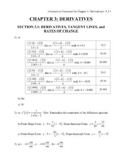
4 ( SECTION : DIFFERENCE QUOTIENTS ) The average velocity is 50 mph on 0, 2 in the three scenarios below. It is the slope of the orange secant line. We will define instantaneous velocity (or simply velocity) in SECTION Here, the velocity is constant (50 mph). Here, the velocity is increasing; the car is accelerating. Here, the car overshoots the destination and then backtracks. WARNING 1: The car s velocity is negative in value when it is backtracking; this happens when the graph falls. In calculus, the Mean Value Theorem for Derivatives will imply that the car must be going exactly 50 mph at some time value t in 0, 2(). The theorem applies in all three scenarios above, because s is continuous on 0, 2 and is differentiable on 0, 2(), meaning that its graph makes no sharp turns and does not exhibit infinite steepness on 0,2().

5 Differentiability will be discussed in SECTION ( SECTION : DIFFERENCE QUOTIENTS ) PART D: FORMS OF DIFFERENCE QUOTIENTS The purposes of these forms will be discussed in SECTION on derivatives. Forms of DIFFERENCE QUOTIENTS Form 1: Fixed interval fb() fa()b a a, b are constants Form 2: Variable endpoint (x) fx() fa()x a a is constant; x is variable Form 3: Variable run (h) fa+h() fa()h a is constant; h is variable Form 4: Variable endpoint (x) and Variable run (h) fx+h() fx()h x, h are variable The denominators can be negative. (See Footnote 2 in SECTION ) ( SECTION : DIFFERENCE QUOTIENTS ) PART E: EVALUATING DIFFERENCE QUOTIENTS Example 2 (Form 1 of a DIFFERENCE Quotient; Profit) A company sells widgets.

6 Assume that all widgets produced are sold. Let P be the profit function for the company; Px() is the profit (in dollars) if x widgets are produced and sold. Our model: Px()= x2+200x 5000. Find the average rate of change of profit between 60 and 90 widgets. WARNING 2: We will treat the domain of P as 0, ), even though one could argue that the domain should only consist of integers. Be aware of this issue with applications such as these. Solution P90() P60()90 60= 90()2+200 90() 5000 60()2+200 60() 5000 30 WARNING 3: Grouping symbols are essential when expanding P60() here, since we are subtracting an expression with more than one term. = 8100+18, 000 5000 3600+12, 000 5000 30= 8100+18, 000 5000+3600 12, 000+500030 TIP 2: Instead of completely evaluating P90() and P60(), it may help to take advantage of cancellations such as the one above.

7 =150030=50dollarswidget ( SECTION : DIFFERENCE QUOTIENTS ) The practical interpretation is that, if the company increases its production level from 60 widgets to 90 widgets, then its profit will increase by 50dollarswidget, on average. The total increase in profit is $1500 over the 30 additional widgets. The graph of y=Px() is below. The slope of the orange secant line is also 50dollarswidget. The fact that the slope is positive reflects the fact that the profit function is increasing on 60, 90 . We will revisit this idea in SECTION on derivatives. ( SECTION : DIFFERENCE QUOTIENTS ) Example 3 (Form 2 of a DIFFERENCE Quotient; Revisiting Example 2 on Profit) Again, Px()= x2+200x 5000.

8 Evaluate Px() P60()x 60. (Form 2) Solution Px() P60()x 60= x2+200x 5000 60()2+200 60() 5000 x 60= x2+200x 5000 3600+12, 000 5000 x 60= x2+200x 5000+3600 12, 000+5000x 60= x2+200x 8400x 60= x2 200x+8400()x 60 The Factor Theorem in Chapter 2 will imply that, if P is polynomial, then x 60() is a factor of the numerator, which is equivalent to Px() P60(). This is because 60 is a zero of the numerator: P60() P60()=0. = x 60()x 140()x 60()1,x 60()= x 140(),x 60()=140 x,x 60() ( SECTION : DIFFERENCE QUOTIENTS ) The unit for the DIFFERENCE quotient is still dollarswidget, though we tend to omit it when a variable is present in our final expression. If we substitute x=90, we obtain 50 dollarswidget , our answer to Example 2.

9 ( SECTION : DIFFERENCE QUOTIENTS ) Example 4 (Form 3 of a DIFFERENCE Quotient; Revisiting Example 2 on Profit) Again, Px()= x2+200x 5000. Evaluate P60+h() P60()h. (Form 3) Solution P60+h() P60()h= 60+h()2+200 60+h() 5000 60()2+200 60() 5000 h= 3600+120h+h2()+12, 000+200h 5000 3600+12, 000 5000 h= 3600 120h h2+12, 000+200h 5000+3600 12, 000+5000h=80h h2h=h80 h()h1,h 0()=80 h,h 0() If we substitute h=30, which corresponds to x=90, we obtain 50 dollarswidget , our answer to Example 2. ( SECTION : DIFFERENCE QUOTIENTS ) Example 5 (Form 4 of a DIFFERENCE Quotient; Revisiting Example 2 on Profit) Again, Px()= x2+200x 5000. Evaluate Px+h() Px()h.

10 (Form 4) Solution Px+h() Px()h= x+h()2+200x+h() 5000 x2+200x 5000 h= x2+2xh+h2()+200x+200h 5000 x2+200x 5000 h= x2 2xh h2+200x+200h 5000 x2+200x 5000 h= x2 2xh h2+200x+200h 5000+x2 200x+5000h= 2xh h2+200hh=h 2x h+200()h1,h 0()= 2x h+200,h 0() If we substitute x=60 and h=30 (which then corresponds to x=90), we obtain 50 dollarswidget , our answer to Example 2. ( SECTION : DIFFERENCE QUOTIENTS ) FOOTNOTES 1. Assumptions made about a function. When defining the average rate of change of a function f on an interval a,b , where a<b, sources typically do not state the assumptions made about f . The formula fb() fa()b a seems only to require the existence of fa() and fb(), but we typically assume more than just that.