Transcription of Simple linear regression - statstutor
1 Simple linear regression Introduction Simple linear regression is a statistical method for obtaining a formula to predict values of one variable from another where there is a causal relationship between the two variables. Straight line formula Central to Simple linear regression is the formula for a straight line that is most commonly represented as cmxy or bxay . Statisticians however generally prefer to use the following form involving betas: xy10 The variables y and x are those whose relationship we are studying. We give them the following names: y: dependent (or response) variable; x: independent (or predictor or explanatory) variable.
2 It is convention when plotting data to put the dependent and independent data on the y and x axis respectively; 0 and 1 are constants and are parameters (or coefficients) that need to be estimated from data. Their roles in the straight line formula are as follows: 0 : intercept; 1 : gradient. For instance the line has an intercept of 1 and a gradient of Its graph is as follows: Model assumptions In Simple linear regression we aim to predict the response for the ith individual, iY, using the individual s score of a single predictor variable, iX.
3 The form of the model is given by: iiiXY 10 which comprises a deterministic component involving the two regression coefficients (0 and 1 ) and a random component involving the residual (error) term (i ). The deterministic component is in the form of a straight line which provides the predicted (mean/expected) response for a given predictor variable value. The residual terms represent the difference between the predicted value and the observed value of an individual. They are assumed to be independently and identically distributed normally with zero mean and variance 2 , and account for natural variability as well as maybe measurement error.
4 Our data should thus appear to be a collection of points that are randomly scattered around a straight line with constant variability along the line: The deterministic component is a linear function of the unknown regression coefficients which need to be estimated so that the model best describes the data. This is achieved mathematically by minimising the sum of the squared residual terms (least squares). The fitting also produces an estimate of the error variance which is necessary for things like significance test regarding the regression coefficients and for producing confidence/prediction intervals.
5 Example Suppose we are interested in predicting the total dissolved solids (TDS) concentrations (mg/L) in a particular river as a function of the discharge flow (m3/s). We have collected data that comprise a sample of 35 observations that were collected over the previous year. The first step is to look carefully at the data: Is there an upwards/downwards trend in the data or could a horizontal line be fit though the data? Is the trend linear or curvilinear? Is there constant variance along the regression line or does it systematically change as the predictor variable changes?
6 The scatterplot above suggests that there is a downwards trend in the data, however there is a curvilinear relationship. The variance about a hypothetical curve appears fairly constant. 02000400060008000 Discharge flow200300400500600700 Total dissolved solids concTransformations Simple linear regression is appropriate for modelling linear trends where the data is uniformly spread around the line. If this is not the case then we should be using other modelling techniques and/or transforming our data to meet the requirements.
7 When considering transformations the following is a guide: If the trend is curvilinear consider a transformation of the predictor variable, x. If constant variance is a problem (and maybe curvilinear as well) consider either a transformation of the response variable, y, or a transformation of both the response and the predictor variable, x and y. Tukey s bulging rule can act as a guide to selecting power transformations. Compare your data to the above and if it has the shape in any of the quadrants then consider the transformations where: up use powers of the variable greater than 1 ( x2, etc); down - powers of the variable less than 1 ( log(x), 1/x, x etc).
8 Note, sometimes a second application of Tukey s bulging rule is necessary to gain linearity with constant variability. (Discharge flow)200300400500600700 Total dissolved solids concExample (revisited) Returning to our example, the scatterplot reveals the data to belong to the bottom left quadrant of Tukey s bulging rule. Since the variance about a hypothetical curve appears fairly constant, thus we shall try transforming just the predictor variable. Tukey s bulging rule suggests a down power; we shall try the log natural transformation first The resulting scatterplot of TDS against ln(Discharge) is now far more satisfactory: The data now appears to be suitable for Simple linear regression and we shall now consider selected output from the statistics package SPSS.
9 The correlations table displays Pearson correlation coefficients, significance values, and the number of cases with non-missing values. As expected we see that we have a strong negative correlation ( ) between the two variables. From the significance test p-value we can see that we have very strong evidence (p< ) to suggest that there is a linear correlation between the two variables. dissolvedsolids concln(Discharge flow)Total dissolvedsolids concln(Discharge flow)Total dissolvedsolids concln(Discharge flow)Pearson CorrelationSig. (1-tailed)NTotaldissolvedsolids concln(Dischargeflow) The model summary table displays: R, the multiple correlation coefficient, is a measure of the strength of the linear relationship between the response variable and the set of explanatory variables.
10 It is the highest possible Simple correlation between the response variable and any linear combination of the explanatory variables. For Simple linear regression where we have just two variables, this is the same as the absolute value of the Pearson s correlation coefficient we have already seen above. However, in multiple regression this allows us to measure the correlation involving the response variable and more than one explanatory variable. R squared is the proportion of variation in the response variable explained by the regression model.