Transcription of Single-Degree-of-Freedom Linear Oscillator (SDOF)
1 Chapter 1 Single-Degree-of-Freedom Linear Oscillator (SDOF) For many dynamic systems the relationship between restoring force and deflection is approximately Linear for small deviations about some reference. If the system is complex ( , a building that requires numerous variables to describe its properties) it is possible to transform it (using the normal modes of the system) into a number of simple 1-dimensional Linear Oscillator problems (SDOF). The SDOF problem is also fundamental to understanding the principles of seismometers. Consider the most fundamental of seismometers shown in Figure ( ). In this case the ground moves with displacement ()ut; a mass is supported by a spring of stiffness k; and there is a viscous damper that resists the relative velocity of the mass with respect to the ground with force.
2 Mx bx ()xt is sometimes measured directly using an optical transducer ( a light beam deflected by a mirror on the mass). the force on is and the inertial force on mkxbx () is mmxu+ . The equation of motion of the system is then ()mxukxbx0,+++= ( ) which can be rewritten as 202xxx u++= , ( ) where 1- 1 0undamped natural frequencykm == ( ) damping constant, 2bm = ( )
3 Which is related to the fraction of critical damping by 0. = ( ) Equation ( ) is a 2nd order Linear differential equation and its solution is widely known. In general the solution is broken into two parts. The homogeneous solution, which solves the equation 202xxx 0++= ( ) Any solutions, xn(t), of the homogeneous equation ( ) can be summed and they also solve the homogeneous equation since it is Linear .
4 The actual form of the solution to the homogeneous problem is determined by the initial conditions 0 0and xx . Solutions to the homogeneous equation can also be summed to solutions to the full inhomogeneous equation ( ) and they will still solve the inhomogeneous equation. The homogeneous solutions typically represent the transient part of the response of the system. The homogeneous solution that matches the initial conditions is then added to the particular solution that solves equation ( ). The particular solution often represents the steady-state part of problems. It is particularly useful to represent the ground motion u(t) as a Fourier series, or ()()(11()cossincosnnnnnnnnutAtBtCt)n == =+= )n ( ) or ()()(2211()cossincosnnnnnnnnnnutAtBtCt == = += ( ) This representation is possible for functions that are periodic with a repeat time of T.
5 In this case 2nnT = ( ) Since our equation is Linear , we can write the solution x(t) as the sum of solutions to individual harmonic problems, or ()()1,nnnxtCxt == ( ) where xn solves the equation 1- 2 ()2202cosnnnnnxxxtn ++= . ( ) Since the cosine function is truly periodic and has no beginning or end, there are no initial conditions or transient solutions to deal with.
6 That is, the solution consists of just the particular solution. As it turns out, when a Linear system is harmonically forced at one frequency, then the resulting motions (except for transients) are also harmonic at that frequency. Therefore, let us guess that the solution of ( ) is ()()cosnnnxtDtn = ( ) substituting ( ) into( ), we find that ()()()(2220cos2sincosnnnnnnnnnnDtDt)t =. ( ) We then utilize the following trig identities ()()()coscoscossinsinnnnnntttn =+ ( ) ()()()sinsincoscossinnnnnntttn = ( ) substituting ( ) and ( ) into ( ) we find that (){}()()()2220220cos2sincossin2cossin0nn nnnnnnnnnnnDtDt + = ) ( ) Now since ()(sin and cosntnt are linearly independent functions, each term in equation ( ) must be linearly independent and thus setting the second term to zero ( )
7 ()220sin2cos0nnnn =or 2202tannnn = ( ) Now setting the first term in( ) to 0 gives ()2220cos2sinnnnnnD n = + ( ) If we make the following clever observation that equation ( ) can be rewritten as the following two equations ()2222202sin4nnnn = + ( ) 1- 3 ()220222220cos4nnnn = + ( ) then we can substitute ( ) and ( ) into ( ) to obtain ()22222204nnnnD = + ( ) thus the steady-state solution of equation ( ) is ()()(2222220cos4nnnnxtt )nnn = + ( ) where, 12202tannnn = ( ) Notice that ()()()0cos when nnxttUtn = ( ) and that ()()
8 ()2020cos when nnnxttUt n = ( ) That is the motion of the mass with respect to the case is proportional to ground displacement at high frequencies and it is proportional to acceleration at low frequencies (compared to the natural frequency). Figure shows the amplitude and phase of xn(t- ) as a function of frequency for an SDOF. Notice that when the damping is 12, then there is the maximum response without having a peak in the response curve. Most manufacturers of seismometers attempt to achieve this level of damping . Figure can be thought of as an amplification factor as a function of frequency for ground acceleration.
9 That is the size of the record x(t) is the ground acceleration times the amplification factor. Notice that the instrument response is proportional to ground acceleration at low frequencies. 1- 4 The amplification can be determined as a function of the amplitude of the ground displacement by simply multiplying the response by 2 . In this case the instrument response looks like Figure Figure Amplification ratio is XU 1- 5 Figure Amplification ratio is XU We can also find the frequency at which the SDOF has its maximum amplitude response to a forced vibration by finding the minimum of the response as follows.
10 0nRnndxd == ( ) where r is the frequency of maximum resonance. Performing this differentiation on equation ( ) gives 220021R22 = = ( ) To add to the things to remember, there is yet another way to describe the system damping called the quality factor Q, which is defined as 21222RQ = ( ) For lightly damped systems, it can be shown that Total Energy in One Cycle12 Energy Loss During One Cycle2Q ( )