Single stub impedance matching Impedance …

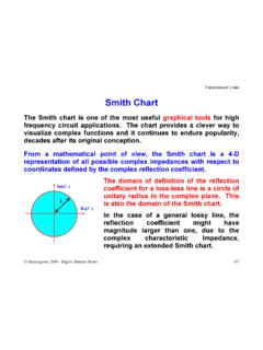
1 Transmission Lines Amanogawa, 2006 Digital Maestro Series 192 Single stub Impedance matching Impedance matching can be achieved by inserting another transmission line ( stub ) as shown in the diagram below ZA = Z0 dstubZRZ0 LstubZ0 STransmission Lines Amanogawa, 2006 Digital Maestro Series 193 There are two design parameters for Single stub matching : The location of the stub with reference to the load dstub The length of the stub line Lstub Any load Impedance can be matched to the line by using Single stub technique. The drawback of this approach is that if the load is changed, the location of insertion may have to be moved.

2 The transmission line realizing the stub is normally terminated by a short or by an open circuit. In many cases it is also convenient to select the same characteristic Impedance used for the main line, although this is not necessary. The choice of open or shorted stub may depend in practice on a number of factors. A short circuited stub is less prone to leakage of electromagnetic radiation and is somewhat easier to realize. On the other hand, an open circuited stub may be more practical for certain types of transmission lines, for example microstrips where one would have to drill the insulating substrate to short circuit the two conductors of the line.

3 Transmission Lines Amanogawa, 2006 Digital Maestro Series 194 Since the circuit is based on insertion of a parallel stub , it is more convenient to work with admittances, rather than impedances. YA = Y0 dstub YR = 1/ZRY0 = 1/Z0 LstubY0 STransmission Lines Amanogawa, 2006 Digital Maestro Series 195 For proper Impedance match: ()stubstub001dAYY YYZ=+ == dstubYR = 1/ZRY (dstub) Lstub Y0S Ystub +Input admittance of the stub line Line admittance at location dstub before the stub is appliedTransmission Lines Amanogawa, 2006 Digital Maestro Series 196In order to complete the design, we have to find an appropriate location for the stub .

4 Note that the input admittance of a stub is always imaginary (inductance if negative, or capacitance if positive) stubstubYjB= A stub should be placed at a location where the line admittance has real part equal to Y0 ()()stub0stubddYYjB=+ For matching , we need to have ()stubstubdBB= Depending on the length of the transmission line, there may be a number of possible locations where a stub can be inserted for Impedance matching . It is very convenient to analyze the possible solutions on a Smith chart. Transmission Lines Amanogawa, 2006 Digital Maestro Series 197 1-10 -332-2zRyR Load location First location suitable for stub insertionSecond location suitable for stub insertiony(dstub1)y(dstub2) Unitary conductance circleConstant | (d)| circle 2 1 Transmission Lines Amanogawa, 2006 Digital Maestro Series 198 The red arrow on the example indicates the load admittance.

5 This provides on the admittance chart the physical reference for the load location on the transmission line. Notice that in this case the load admittance falls outside the unitary conductance circle. If one moves from load to generator on the line, the corresponding chart location moves from the reference point, in clockwise motion, according to an angle (indicated by the light green arc) 42dd = = The value of the admittance rides on the red circle which corresponds to constant magnitude of the line reflection coefficient, | (d)|=| R |, imposed by the load. Every circle of constant | (d)| intersects the circle Re { y } = 1 (unitary normalized conductance), in correspondence of two points.

6 Within the first revolution, the two intersections provide the locations closest to the load for possible stub insertion. Transmission Lines Amanogawa, 2006 Digital Maestro Series 199 The first solution corresponds to an admittance value with positive imaginary part, in the upper portion of the chart ()()() ()()111stub0stub1stubstub111stubstubdd d1dd4dYYjByjbjB=+=+ = Line Admittance - Actual :Normalized : stub Location : stub Admittance - Actual : Norma()()()()111stub1stub0stub1stub0stub d1tan()2dtand()2ssjbLZBLZB = = lized : stub Length :shortopenTransmission Lines Amanogawa, 2006 Digital Maestro Series 200 The second solution corresponds to an admittance value with negative imaginary part, in the lower portion of the chart ()()() ()()222stub0stub2stubstub222stubstubdd d1dd4dYYjByjbjB= = = Line Admittance - Actual :Normalized : stub Location : stub Admittance - Actual : Norma()()()()222stub1stub0stub1stub0stub d1tan()2dtand()2ssjbLZBLZB = = lized : stub Length.

7 Shortopen Transmission Lines Amanogawa, 2006 Digital Maestro Series 201If the normalized load admittance falls inside the unitary conductance circle (see next figure), the first possible stub location corresponds to a line admittance with negative imaginary part. The second possible location has line admittance with positive imaginary part. In this case, the formulae given above for first and second solution exchange place. If one moves further away from the load, other suitable locations for stub insertion are found by moving toward the generator, at distances multiple of half a wavelength from the original solutions.

8 These locations correspond to the same points on the Smith chart. 12stubstubd2d2nn= =+ +First set of locationsSecond set of locations Transmission Lines Amanogawa, 2006 Digital Maestro Series 202 1-10 -332-2 yRzR Load locationSecond location suitable for stub insertionFirst location suitable for stub insertiony(dstub2)y(dstub1) Unitary conductance circleConstant | (d)| circle 2 1 Transmission Lines Amanogawa, 2006 Digital Maestro Series 203 Single stub matching problems can be solved on the Smith chart graphically, using a compass and a ruler. This is a step-by-step summary of the procedure: (a) Find the normalized load Impedance and determine the corresponding location on the chart.

9 (b) Draw the circle of constant magnitude of the reflection coefficient | | for the given load. (c) Determine the normalized load admittance on the chart. This is obtained by rotating 180 on the constant | | circle, from the load Impedance point. From now on, all values read on the chart are normalized admittances. Transmission Lines Amanogawa, 2006 Digital Maestro Series 204 1-10 -332-2 zRyR (c) Find the normalized load admittance knowing that yR = z(d= /4 ) From now on the chart represents admittances. (a) Obtain the normalized load Impedance zR=ZR /Z0 and find its location on the Smith chart (b) Draw the constant | (d)|circle 180 = /4 Transmission Lines Amanogawa, 2006 Digital Maestro Series 205(d) Move from load admittance toward generator by riding on the constant | | circle, until the intersections with the unitary normalized conductance circle are found.

10 These intersections correspond to possible locations for stub insertion. Commercial Smith charts provide graduations to determine the angles of rotation as well as the distances from the load in units of wavelength. (e) Read the line normalized admittance in correspondence of the stub insertion locations determined in (d). These values will always be of the form ()()stubstubd1 top half of chartd1 bottom half of chartyjbyjb=+= Transmission Lines Amanogawa, 2006 Digital Maestro Series 206 1-10 zRyR Load location First location suitable for stub insertion dstub1=( 1/4 ) 1(d) Move from load toward generator and stop at a location where the real part of the normalized line admittance is conductance circle(e) Read here the value of the normalized line admittance y(dstub1)