Transcription of SOLUTIONS FOR HOMEWORK SECTION 6.4 AND 6.5 …
1 SOLUTIONS FOR HOMEWORK SECTION AND Problem 1: For each of the following functions do the following: (i) Write the function as a piecewise function and sketch its graph, (ii) Write the function as a combination of terms of the form ua (t)k(t a) and compute the Laplace transform (a) f (t) = t(1 u1 (t)) + et (u1 (t) u2 (t)). (b) h(t) = sin(2t) + u (t)(t/ sin(2t)) + u2 (t)(2 t)/ . (c) g(t) = u0 (t) + 5k=1 ( 1)k uk (t). P. Solution: (a).. t 0 t<1. f (t) = et 1 t < 2. 0 t 2.. The graph is sketched in figure 1. Figure 1. graph of f(t). To find the Laplace transform of f (t), rewrite f (t) as f (t) = t + (et t)u1 (t) et u2 (t). L{f } = L{t} + L{et u1 (t)} L{tu1 (t)} L{et u2 (t)}.
2 1. SOLUTIONS FOR HOMEWORK SECTION AND 2. Apply t-shifting theorem (Theorem in the textbook) or s-shifting theorem if needed, finding the Laplace transform for each term: 1. L{t} = 2. s e(1 s). L{et u1 (t)} = eL{e(t 1) u1 (t)} = e e s L{et } =. s 1. s e e s L{tu1 (t)} = L{(t 1)u1 (t)} + L{u1 (t)} = 2 +. s s (2 2s). e L{et u2 (t)} = e2 L{e(t 2) u2 (t)} = e2 e 2s L{et } =. s 1. Combining all terms yields 1 e(1 s) e s e s e(2 2s). L{f } = + 2 . s2 s 1 s s s 1. (b) . sin(2t) 0 t . h(t) = t/ t < 2 . 2 2.. The graph is sketched in figure 2. Figure 2. graph of h(t). To find the Laplace transform of h(t), L{h} = L{sin(2t)} + L{u (t)(t/ sin(2t))} + L{u2 (t)(2 t)/ }.
3 Apply t-shifting theorem if needed, and find the Laplace transform of each term: 2. L{sin(2t)} = 2. s +4. SOLUTIONS FOR HOMEWORK SECTION AND 3. t+ 1 1 2. L{u (t)(t/ sin(2t))} = e s L{( sin(2(t + )))} = e s ( 2 + 2 ). s s s +4. 2 (t + 2 ) 1. L{u2 (t)(2 t)/ } = e 2 s L{ } = e 2 s 2. s Combining all terms yields 2 1 1 2 1. L{h} = 2 + e s ( 2 + 2 ) e 2 s 2. s +4 s s s +4 s (c) Here u0 (t) = 1 since we are only interested in the domain t 0. 1 0 t<1.. 0 1 t<2.. 1 2 t<3.. g(t) =.. 0 3 t<4. 1 4 t<5.. 0 t 5. The graph is sketched in figure 3. Figure 3. graph of g(t). To find the Laplace transform of g(t), 5. X. L{g} = L{1} + L{( 1)k uk (t)}.
4 K=1. 5. 1 X e ks = + ( 1)k s k=1 s 1 e s e 2s e 3s e 4s e 5s = + + . s s s s s s Problem 2: Solve the initial value problem . 0 if 0 t < 1. 0. y + 6y = g(t) where g(t) = 12 if 1 t < 7. 0 if 0 t SOLUTIONS FOR HOMEWORK SECTION AND 4. with initial value y(0) = 4. Solution: Use step function to represent g(t) as g(t) = 12(u1 (t) u7 (t)). Take the Laplace transform of the differential equation and plug in initial value to get e s e 7s sY (s) 4 + 6Y (s) = 12( ). s s Solving for Y (s) yields 12e s 12e 7s 4. Y (s) = +. s(s + 6) s(s + 6) s + 6. 1. Let H(s) = s(s+6) , by partial fraction, we can rewrite H(s) as 1 1 1. H(s) = ( ). 6 s s+6.
5 The inverse Laplace transform of H(s) is 1. h(t) = L 1 {H} = (1 e 6t ). 6. Hence, by using t-shifting theorem if necessary, we can find the solution y(t) = L{Y } = 12u1 (t)h(t 1) 12u7 (t)h(t 7) + 4e 6t Problem 3: Solve the initial value problem . 00 t if 0 t < 1. y + y = g(t) where g(t) =. 0 if 1 t and with y(0) = 0 and y 0 (0) = 0. Solution: Firstly we can rewrite g(t) as g(t) = t(1 u1 (t)). To find the Laplace transform of g(t), we need use t-shifting theorem 1 1 1 1. L{g(t)} = L{t} L{u1 (t)t} = e s L{t + 1} = e s ( 2 + ). s s s s Then take the Laplace transform of the differential equation and plug in initial values to get 1 e s e s s2 Y (s) + Y (s) = 2.
6 S s s Solving for Y (s) yields 1 e s e s Y (s) = . s(s2 + 1) s(s2 + 1) s2 (s2 + 1). SOLUTIONS FOR HOMEWORK SECTION AND 5. Let 1 1. H(s) = and F (s) = 2 2. s(s2. + 1) s (s + 1). We could use the method of undetermined coefficients method to find the partial fraction for H(s): 1 s 1 1. H(s) = 2 and F (s) = 2 2. s s +1 s s +1. The inverse Laplace transform of them are h(t) = 1 cos(t) and f (t) = t sin(t). By applying t-shifting theorem if necessary, the inverse Laplace transform of Y (s) is: y(t) = L{H(s)} L{e s H(s)} L{e s F (s)}. = h(t) u1 (t)h(t 1) u1 (t)f (t 1). Problem 4: Consider the mass-spring system described by the initial value problem y 00 + 4y = sin t + u /2 (t) cos t; y(0) = 0, y 0 (0) = 0.
7 Find the solution of the initial value problem. Hint: Rewrite cos t using a trigonometric identity. Solution: First need to write u /2 (t) cos t in the form uc (t)f (t c). To do this use the trig identities cos = sin( /2 ) and sin( ) = sin . This gives . u /2 (t) cos t = u /2 (t) sin t = u /2 (t) sin t . 2 2. Substituting this into the ODE and taking the Laplace transform gives us . 2 1 e 2 s (s + 4)Y (s) = 2 2. s +1 s +1. Solving for Y yields 1 2 s Y (s) = (1 e ). (s2 + 1)(s2 + 4). Let 1. H(s) =. (s2 + 1)(s2 + 4). We use partial fractions to rewrite H: 1 As + B Cs + D. 2 2. = 2 + 2. (s + 1)(s + 4) s +4 s +1. = 1 = (As + B)(s + 1) + (Cs + D)(s2 + 4).
8 2. = 1 = (A + C)s3 + (B + D)s2 + (A + 4C)s + (B + 4D). Equating coefficients yields the four equations A + C = 0, B + D = 0, A + 4C = 0, B + 4D = 1. SOLUTIONS FOR HOMEWORK SECTION AND 6. which has the solution A = C = 0, B = 1/3 and D = 1/3. Therefore we can write 1 2 1 1. H(s) = 2 + 2. 6 s +4 3s +1. and so 1 1. h(t) = L 1 {H} = sin(2t) + sin(t). 6 3. It follows (using the t-shifting theorem where necessary) that y(t) = h(t) u /2 (t)h(t /2). Problem 5: Determine the value of the following integrals R7. (a) 2 (t + 1) dt. R7. (b) 2 (t 1) dt. R8. (c) 1 ln (t2 ) (t e) dt. R4. (d) 2 (2t4 t3 + 7t2 1) (t 5) dt. Solution: To evaluate the above integrals, we will be using the well-known formula derived in class which is given by Z.
9 (t t0 )f (t) dt = f (t0 ).. It should be noted in passing that the value of t0 must lie within the interval of integration. Otherwise, the value of the definite integral will be zero. (a) 0. (b) 1. (c) 2. (d) 0. Problem 6: Find the solution of the initial value problem and sketch the graph of the solution for y 00 + 2y 0 + 2y = (t ); y(0) = 1, y 0 (0) = 0. ( ). Solution: SOLUTIONS FOR HOMEWORK SECTION AND 7. Let us take initially the Laplace transform of the IVP given and solve for Y (s) = L{y(t)}. afterwards: s+2 e s s2 Y s + 2sY 2 + 2Y = e s Y = 2 + 2 . s + 2s + 2 s + 2s + 2. s+2 e s Y = + . (s + 1)2 + 1 (s + 1)2 + 1. s+1 1 e s Y = + +.
10 ( ). (s + 1)2 + 1 (s + 1)2 + 1 (s + 1)2 + 1. Next, note that the inverse of the first two terms in Eq. ( ) can be obtained by utilizing the s-shifting theorem, that is, ( ) 1. s+1 n s o 1. t L = e L 2 = e t cos (t), ( ). (s + 1)2 + 1 s +1. ( ) 1. 1 n 1 o 1. t L 2 = e L 2+1. = e t sin (t). ( ). (s + 1) + 1 s Note that we could use the formulas 9 and 10 in 252 in the textbook for the above inverses. Finally, and as far as the last term in Eq. ( ) is concerned, we will apply a combination of the t- and s- shifting theorems: ( ) 1 ( ) 1. e s s L = L H(s + 1)e = u (t)h(t ), ( ). (s + 1)2 + 1. where h(t) = e t sin (t) and u represents the Heaviside function for c =.
![[Chapter 5. Multivariate Probability Distributions]](/cache/preview/1/5/9/1/5/3/9/b/thumb-1591539b1a407f741d1c8ef6013023a0.jpg)