Transcription of Solving Differential Equations Using Simulink
1 R . H E R M A NS O LV I N G D I F F E R E N T I A L E Q UAT I O N SU S I N G S I M U L I N KR . L . H E R M A N - V E R S I O N DAT E : J U LY 1 , 2 0 1 9 Copyright 2019by R. Hermanpublished by text has been reformatted from the original Using a modification of the Tufte-book documentclass in Differential Equations Using simulinkby Russell Herman is licensed under a Creative Com-mons Attribution-Noncommercial-Share States License. These notes have resided printing,2015 Contents1 Introduction to Simulink11 Solving an ODE ..12 Handling Time in First Order Differential Equations ..83 Working with Simulink Output ..134 Printing Simulink Scope Images ..145 Scilab and Xcos ..196 First Order ODEs in MATLAB.
2 21 Symbolic Solutions ..22 ODE45and Other Solvers..23 Direction Fields ..237 Exercises ..262 First Order Differential Equations271 Exponential Growth and Decay ..272 Newton s Law of Cooling ..293 Free Fall with Drag ..334 Pursuit Curves ..355 The Logistic Equation ..386 The Logistic Equation with Delay ..397 Exercises ..413 Second Order Differential Equations431 Constant Coefficient Equations ..44 Harmonic Oscillation ..452 Projectile Motion ..543 The Bouncing Ball ..564 Nonlinear Pendulum Animation ..595 Second Order ODEs in MATLAB ..626 Exercises ..664 Transfer Functions and State Space Blocks691 State Space Formulation ..692 Transfer Functions ..7045 Systems of Differential Equations731 Linear Systems.
3 732 Nonlinear Models ..756 Index831 Introduction to SimulinkThere are several computer packagesfor finding solutions of dif-Most of these models were createdusing Version2015. Some changes inVersions2017-2018are Equations , such as Maple, Mathematica, Maxima, MATLAB, systems provide both symbolic and numeric approaches to findingsolutions. They often require a bit of coding. However, there are graphicalenvironments for Solving problems, including Differential Equations . Onesuch environment is Simulink , which is closely connected to MATLAB. Inthese notes we will first lead the reader through examples of solutions offirst and second order Differential Equations usually encountered in a dif-ferential Equations course Using Simulink .
4 We will then look at examplesof more complicated an ODES imulink is a graphical environmentfor designing simulationsof systems. As an example, we will use Simulink to solve the first orderdifferential equation (ODE)dxdt=2 sin 3t 4x.( )We will also need an initial condition of the formx(t0) =x0att=t0. Forthis problem we will letx(0) = can solve Equation ( ) by integratingdxdtto formally obtainx(t) = (2 sin 3t 4x(t)) will view this as a system in which the input,x =2 sin 3t 4x, is fedinto an integrator and the output will bex(t). Generally, we havex(t) = x (t) process is depicted in outputxx : Schematic for a generalsystem in which the block takes theinput and produces an order to carry this out, we separately insert the terms 2 sin 3tand 4xinto the integration procedure.
5 Since we do not know 4x, we take2 Solving Differential Equations Using simulinkthe output from the integrator, multiply it by 4, and subtract that from2 sin 3t. This combined set of terms is then feed back into the is shown schematically in sin 3t output 4+ xx : Schematic for solvingx =2 sin 3t 4x. The terms 2 sin 3tand4xare fed into the integrator you have access to Simulink and MATLAB, you can start MAT-LAB by typingsimulinkon the command line to bring up Simulink . Al-ternatively, you can select Simulink on the MATLAB icon bar to launchSimulink. Starting in2017 Simulink opens with a start screen in whichthere are several selections as shown in the Blank Model1In earlier versions the Simulink Li-brary Browser in begin a new model or select a recently opened model.
6 Then, you will bein the Simulink workspace [see ]. : The Simulink Start the Blank Model to begin a newmodel or select a recently the workspace you can open the Simulink Library Browser asshown in Next, click the yellow plus to bring up a new build models by dragging and connecting the needed components, orblocks, from groups such as the Continuous, Math Operations, Sinks, we can create the model for simulating Equation ( ) in Simulinkas described in Figure schema2using Simulink blocks and a differentialequation (ODE) solver. In the background Simulink uses one of MAT-LAB s ODE solvers, numerical routines for Solving first order differentialequations, such asode45. This system uses theIntegratorblock31sIntegratorto3 The notation on theIntegratorblock isrelated to the Laplace transformL[ t0f( )d =1sF(s),]whereF(s)is the Laplace transform off(t).
7 Integratedxdt, producingx(t).introduction to Simulink : A blank model in : The Simulink LibraryBrowser. This is where various blockscan be found for constructing models.[As seen in MATLAB2015a.]The input for theIntegratoris the right side of the Differential Equation( ), 2 sin 3t 4x. The sine function can be provided by Using theSineWaveblock, whose parameters are set in theSine Waveblock. In order toget 4x, we grab the output of theIntegrator(x) and boost it by changing4 Solving Differential Equations Using simulinkthe Gain value to "4." Then, Using theSumcomponent, these terms areadded, or subtracted, and fed into the integrator. TheScopeis used toplot the output of theIntegratorblock,x(t). That is the main idea behindsolving this system Using the model in : System for Solving firstorder ODEdxdt=2 sin 3t 4xas aSimulink this example, we implement the following detailed steps in Simulink : Drag needed blocks into the model region [ ]: Integratorblock from the Continuous group; Sumblock from the Math Operations group, Gainblock from the Math Operations group, Sine Waveblock from the Math Operations group; and, Scopeblock from the Sink : Add needed components tothe model window.
8 Connect the output of theSumblock to the input of theIntegratorblock. [ ]1sIntegratorScopeSine Wave1sIntegratorScopeSine : Example of connectingtwo components: Align the compo-nents, Click on output of one and dragto another. Then, release to finalizeconnection. Sometimes it is easier todouble-click the temporary arrow toconnect the blocks. Connect theIntegratorto theScopeby clicking on theIntegratorout-put and dragging to theScopeuntil they are connected. In more recentversions it is easier to double-click the unattached arrow to get a con-nection. Right-click theGaincontrol and chooseFlip BlockunderRotate &Flip. Double-click theGainblock and change theGainblock valuefrom1to4. It should change on the to Simulink : Block Parameters for theSumcontrol.
9 In many cases it is best toalso select the rectangular shape overthe default round shape. Double-click theSumcontrol to bring upBlock Parametersas shown change from |++ to |+- in order to set addition/subtractionnodes. [Note that the symbol | is a blank node. Also, one can changethe block to rectangular form. This is often useful in displaying an over-all flow direction to the model. In this case the spacer, |, is not needed.] Double-click theSine Waveblock and change the frequency to3rad/sand the amplitude to2. [See ] Set the time dropdown menutoUse Simulation : Parameters for theSineWaveblock. Select the amplitude andfrequency Solving Differential Equations Using Simulink Connect theGainoutput to the negative input ofSumand theSineWaveoutput to the positive input on the Sum control.
10 [Note: The Gaincan be set to a negative value and connected to a + node in theSumblock to obtain the same effect.] To add a node to route anxvalue to theGain, hold theCTRL keyandclick on the Output line of theIntegratorand drag towards the inputof theGain. You can also Right-Click the line where you want the nodeand drag from there to theGainblock. See : Add a node by right-clicking one the line and dragging tothe input of a block. The initial value,x(0), ofxis inserted by double-clicking theIntegratorand setting the value. For this example we setx(0) =0. One can annotate the diagram by clicking near where labels are neededand typing in the text box. This leads to the model in Inmore current versions the default is to hide block Release2017b the names of blocksare hidden.