Transcription of Solving Systems of Linear Equations Using Matrices
1 Provided by the Academic Center for Excellence 1 Solving Systems of Linear Equations Using Matrices Summer 2014 Solving Systems of Linear Equations Using Matrices What is a Matrix? A matrix is a compact grid or array of numbers. It can be created from a system of Equations and used to solve the system of Equations . Matrices have many applications in science, engineering, and math courses. This handout will focus on how to solve a system of Linear Equations Using Matrices . How to Solve a System of Equations Using Matrices Matrices are useful for Solving Systems of Equations . There are two main methods of Solving Systems of Equations : Gaussian elimination and Gauss-Jordan elimination. Both processes begin the same way. To begin Solving a system of Equations with either method, the Equations are first changed into a matrix.
2 The coefficient matrix is a matrix comprised of the coefficients of the variables which is written such that each row represents one equation and each column contains the coefficients for the same variable in each equation. The constant matrix is the solution to each of the Equations written in a single column and in the same order as the rows of the coefficient matrix. The augmented matrix is the coefficient matrix with the constant matrix as the last column. Example: Write the coefficient matrix, constant matrix, and augmented matrix for the following system of Equations : 3 2 + 4 = 9 3 2 = 5 4 3 + 2 = 7 Solution: The coefficient matrix is created by taking the coefficients of each variable and entering them into each row. The first equation will be the first row; the second equation will be the second row, and the third equation will be the third row.
3 Also, the first column will represent the variable; the second column will represent the variable, and the third column will represent the variable. 3 2403 24 32 Provided by the Academic Center for Excellence 2 Solving Systems of Linear Equations Using Matrices Summer 2014 Because the second equation does not contain an variable, a 0 has been entered into the column in the second row. The constant matrix is a single column matrix consisting of the solutions to the Equations . 957 To create the augmented matrix, add the constant matrix as the last column of the coefficient matrix. 3 24903 254 327 For the Gaussian elimination method, once the augmented matrix has been created, use elementary row operations to reduce the matrix to Row-Echelon form.
4 There are three basic types of elementary row operations: (1) row swapping, (2) row multiplication, and (3) row addition. Row multiplication and row addition can be combined together. (1) In row swapping, the rows exchange positions within the matrix. The matrix resulting from a row operation or sequence of row operations is called row equivalent to the original matrix. Example: Swap row one and row three Solution: 3 24903 254 327 1 3 4 32703 25 3 249 (2) In row multiplication, every entry in a row is multiplied by the same constant. Example: Multiply row one by 13 Solution: 3 24903 254 327 1 3 1 12/3 4/3 303 254 327 Provided by the Academic Center for Excellence 3 Solving Systems of Linear Equations Using Matrices Summer 2014 (3) In row addition, the column elements of row A are added to the column elements of row B.
5 The resulting sums replace the column elements of row B while row A remains unchanged. Example: Add row one to row two Solution: 3 24903 254 327 1+ 2 3 2 490 +( 3)3 +( 2) 2 + 45 + 94 3 27 3 249 312144 327 The previous examples all started from the original augmented matrix. In order to solve a system of Equations , these row operations are performed back to back on the resulting matrix, instead of returning to the original matrix each time, until Row-Echelon form is achieved. Row-Echelon form is characterized by having the furthest left non-zero entry in a row, the leading entry, with all zeros below it, and the leading entry of each row is in a column to the right of the leading entry in the row above it. For Pre-Calculus students, the leading entry in each row should be reduced to a 1; for Linear Algebra students, this leading entry could be any number unless otherwise specified in your assignment.
6 Example: Are the following Matrices in Row-Echelon form? a) 1 9270014017 6 b) 16 811011 30001 c) 151201 7001 Solution a): No, this matrix is not in Row-Echelon form since the leading entry in row three is in a column to the left of the leading entry in row two. Please note: If we swapped row two and row three, then the matrix would be in Row-Echelon form. Provided by the Academic Center for Excellence 4 Solving Systems of Linear Equations Using Matrices Summer 2014 Solution b): Yes, this matrix is in Row-Echelon form as the leading entry in each row has 0 s below, and the leading entry in each row is to the right of the leading entry in the row above. Notice the leading entry for row three is in column 4 not column 3. The leading entry is allowed to skip columns, but it cannot be to the left of the leading entry in any row above it.
7 Solution c): Yes, this matrix is in Row-Echelon form. Each leading entry in each row is to the right of the leading entry in the row above it, and each leading entry contains only 0 s below it. The following example will demonstrate how to use the elementary row operations to reduce the augmented matrix from a system of Equations to Row-Echelon form. After Row-Echelon form is achieved, back substitution can be used to find the solution to the system of Equations . Example: Solve the following system of Equations Using Gaussian Elimination: 3 2 + 4 = 9 3 2 = 5 4 3 + 2 = 7 Solution: First, create the augmented matrix for the system. 3 24903 254 327 Next use the elementary row operations to reduce the matrix to Row-Echelon form. 3 24903 254 327 13 1 123 43 303 254 327 4 1+ 3 123 43 303 250 17322319 317 3 123 43 303 2501 2217 5717 3 2 123 43 301 2217 571703 25 3 2+ 3 123 43 301 2217 571700321725617 1732 3 Provided by the Academic Center for Excellence 5 Solving Systems of Linear Equations Using Matrices Summer 2014 123 43 301 2217 57170018 Finally, rewrite the matrix as a system of reduced Equations and back substitute to find the solution.
8 1 +23 43 = 3 1 2217 = 5717 1 = 8 The reduced Equations show that = 8. Substitute 8 for and solve for in the second equation. 1 2217(8) = 5717 17617= 5717 = 7 Substitute 8 for and 7 for in the first equation and solve for . +23(7) 43(8) = 3 +143 323= 3 6 = 3 = 3 The solution to the system of Equations is (3,7,8). An alternative method, the Gauss-Jordan elimination method, can be used to solve the system of Equations . This involves reducing the augmented matrix to Reduced Row-Echelon form. The Reduced Row-Echelon form is similar to the Row-Echelon form except that the leading entry in each row must be a 1 and all other entries in the same column as a leading entry must be 0. Unlike the Row-Echelon form, there is one and only one Reduced Row-Echelon form for a system of Equations .
9 Example: Solve the following system of Equations Using Gauss-Jordan Elimination: 3 2 + 4 = 9 Provided by the Academic Center for Excellence 6 Solving Systems of Linear Equations Using Matrices Summer 2014 3 2 = 5 4 3 + 2 = 7 Solution: First, create the augmented matrix for the system. 3 24903 254 327 Next, use the elementary row operations to reduce the matrix to Reduced Row-Echelon form. 3 24903 254 327 13 1 123 43 303 254 327 4 1+ 3 123 43 303 250 17322319 317 3 123 43 303 2501 2217 5717 3 2 123 43 301 2217 571703 25 3 2+ 3 123 43 301 2217 571700321725617 1732 3 123 43 301 2217 57170018 2217 3+ 2 123 43 301070018 43 3+ 1 123023301070018 23 2+ 1 100301070018 The solution to the system can be written directly from the Reduced Row-Echelon form by converting the matrix back to equation form.
10 = 3 = 7 = 8 Thus, the solution to the system of Equations is (3,7,8). This is the same solution obtained by Using the Gaussian elimination method in the previous example. The system of Equations above is an example of a consistent system of Equations . A consistent system of Equations is characterized by having a leading coefficient in each column of the coefficient matrix Provided by the Academic Center for Excellence 7 Solving Systems of Linear Equations Using Matrices Summer 2014 when it is row reduced to either Row-Echelon form or Reduced Row-Echelon form. In other words, each variable represented by a column can be solved for a specific number. With an inconsistent system of Equations , the leading coefficient in one of the rows will be in the last column of the augmented matrix.