Transcription of Spherical Harmonics - Department of Computer Science
1 Spherical Harmonics B. S. PHERICAL Harmonics are a frequency-space basis for representing functions defined over the sphere. They are the Spherical analogue of the 1D Fourier series. Spherical Harmonics arise in many physical problems ranging from the computation of atomic electron configurations to the representation of gravitational and magnetic fields of planetary bodies. They also appear in the solutions of the Schr dinger equation in Spherical coordinates. Spherical Harmonics are therefore often covered in textbooks from these fields [MacRobert and Sneddon, 1967; Tinkham, 2003]. Spherical Harmonics also have direct applicability in Computer graphics. Light transport involves many quantities defined over the Spherical and hemispherical domains, making Spherical Harmonics a natural basis for representing these functions . Early applications of Spherical har- monics to Computer graphics include the work by Cabral et al.
2 [1987] and Sillion et al. [1991]. More recently, several in-depth introductions have appeared in the graphics literature [Ramamoorthi, 2002; Green, 2003; Wyman, 2004; Sloan, 2008]. In this appendix, we briefly review the Spherical Harmonics as they relate to Computer graphics. We define the basis and examine several important properties arising from this defini- tion. 167. 168. Definition A harmonic is a function that satisfies Laplace's equation: 2 f = 0. ( ). As their name suggests, the Spherical Harmonics are an infinite set of harmonic functions defined on the sphere. They arise from solving the angular portion of Laplace's equation in Spherical coordinates using separation of variables. The Spherical harmonic basis functions derived in this fashion take on complex values, but a complementary, strictly real-valued, set of Harmonics can also be defined. Since in Computer graphics we typically only encounter real-valued functions , we restrict our discussion to the real-valued basis.
3 If we represent a direction vector ~. using the standard Spherical parameterization, ~. = sin cos , sin sin , cos , . ( ). then the real Spherical harmonic basis functions are defined as: p m . m 2K l cos(m )P l (cos ) if m > 0, .. m y l ( , ) = K 0 P 0 (cos ) if m = 0, ( ). l l . p m 2K sin( m )P m (cos ) if m < 0.. l l where K lm are the normalization constants s (2l + 1) (l |m|)! K lm = , ( ). 4 (l + |m|)! and P lm are the associated Legendre polynomials. There are many ways to define the associated Legendre polynomials but the most numerically robust way to evaluate them is using a set of 169. recurrence relations [Press et al., 1992]1 : P 00 (z) = 1, ( ). m Pm (z) = (2m 1)!!(1 z 2 )m/2 , ( ). m m P m+1 (z) = z(2m + 1)P m (z), ( ). z(2l 1) m (l + m 1) m P lm (z) = P l 1 (z) P l 2 (z). ( ). l m l m The basis functions are indexed according to two integer constants, the order, l , and the degree, m 2 . These satisfy the constraint that l N and l m l ; thus, there are 2l + 1 basis functions of order l.
4 The order l determines the frequency of the basis functions over the sphere. The Spherical Harmonics may be written either as trigonometric functions of the Spherical coordinates and as above, or alternately as polynomials of the cartesian coordinates x, y, and z. Using the cartesian representation, each y lm for a fixed l corresponds to a polynomial of maximum order l in x, y, and z. 1 We omit the Condon-Shortley phase factor [Condon and Shortley, 1951] of ( 1)m which is sometimes includes in the definition of P lm or y lm since this simplifies our notation. 2 The order l is also sometimes refered to as the band index, and in quantum mechanics, l and m are refered to as quantum numbers and the Spherical Harmonics states.. 170. The first few Spherical Harmonics , in both Spherical and cartesian coordinates, expand to: Spherical Cartesian r r 1 1. l =0 y 00 ( , ) = , 4 4 . r r 3 3. y 1 1 ( , ) = sin sin x.
5 4 4 . r r 3 3.. l =1 y 10 ( , ) = cos z, .. 4 4 . r r 3 3.. y 1 ( , ) =.. cos sin y, . 1. 4 4 . r r 15 15. y 2 2 ( , ) = sin cos sin2 .. x y, 4 4 .. r r 15 15. y 2 1 ( , ) = sin sin cos .. y z, .. 4 4 . r r 5 5.. l =2 y 20 ( , ) = (3 cos2 1) (3z 2 1), .. 16 16 . r r 15 15.. 1.. y 2 ( , ) = cos sin cos xz, .. 4 8 . r r 15 15 2.. y 2 ( , ) = (cos2 sin2 ) sin2 (x y 2 ).. 2. 16 32 . We illustrate the first basis functions in Figure Projection and Expansion The Spherical Harmonics define a complete basis over the sphere. Thus, any real-valued Spherical function f may be expanded as a linear combination of the basis functions l X. ) = y lm (~. ) f lm , X. f (~ ( ). l =0 m= l where the coefficients f lm are computed by projecting f onto each basis function y lm Z. f lm = y lm (~. ) f (~. )d~.. ( ). 4 . Just as with the Fourier series, this expansion is exact as long as l goes to infinity; however, this requires an infinite number of coefficients.
6 By limiting the number of bands to l = n 1 we retain 171. y 00. y 1 1 y 10 y 11. y 2 2 y 2 1 y 20 y 21 y 22. Figure : Plots of the real-valued Spherical harmonic basis functions . Green indicates positive values and red indicates negative values. only the frequencies of the function up to some threshold, obtaining an n th order band-limited approximation f of the original function f : n 1 l f (~. ) = y lm (~. ) f lm . X X. ( ). l =0 m= l Low-frequency functions can be well approximated using only a few bands, and as the number of coefficients increases, higher frequency signals can be approximated more accurately. It is often convenient to reformulate the indexing scheme to use a single parameter i = l (l + 1) + m. With this convension it is easy to see that an n th order approximation can be reconstructed using n 2 coefficients, 2. nX 1. f (~. ) = ) f i . y i (~ ( ). i =0. 172. Properties The Spherical harmonic functions have many basic properties that make them particularly convenient for use in Computer graphics.
7 1. Convolution. Since the Spherical harmonic basis is effectively a Fourier domain basis defined over the sphere, it inherits a similar frequency space convolution property. If h(z) is a circularly symmetric kernel, then the convolution h ? f is equivalent to weighted multiplication in the SH domain r 4 0 m (h ? f )m = h f . ( ). l 2l + 1 l l The convolution property allows for efficient computation of prefiltered environment maps and irradiance environment maps [Ramamoorthi and Hanrahan, 2001]. 2. Orthonormality. The Spherical Harmonics are orthogonal for different l and different m. This means that the inner product of any two distinct basis functions is zero. Furthermore, the normalization constant K lm ensures that the inner product of a basis function with itself is one. This can be expressed mathematically as Z. ) y j (~. y i (~ )d~. = i j , ( ). 4 . where i j is the Kronecker delta function. The efficient projection and expansion operations described above are made possible by the fact that the SH basis is orthonormal.
8 Many other useful and efficient operations also result from this important property. 3. Double Product Integral. The orthonormality property provides for a very simple expres- sion to compute the integrated product of two functions represented in the SH basis. The 173. ) and b (~. integral product of two SH functions a (~ ) can be expanded as Z Z ! ! ) b (~. )d~. = ) ) d~. , X X. a (~ a i y i (~ b j y j (~ ( ). 4 4 i j Z. ) y j (~. )d~. , XX. = ai b j y i (~ ( ). i j 4 . | {z }. Ci j where C i j are called the coupling coefficients, which, due to the definition of orthonormal- ity in Equation , are simply C i j = i j . This simple form for the coupling coefficients introduces significant sparsity in the expression above, leading to the simplification: Z. ) b (~. )d~. =. XX. a (~ ai b j C i j , ( ). 4 i j a i b j i j , XX. = ( ). i j X. = ai bi . ( ). i This expression states that the integrated product of two SH functions is simply the dot product of their coefficient vectors.
9 The double product integral is of particular interest in Computer graphics since it means lighting can be computed very efficiently in the frequency domain. If both the lighting and the cosine-weighted BRDF are represented in the SH basis, then the lighting integral can be computed using a simple dot product. This property is exploited by many PRT techniques [Sloan et al., 2002; Kautz et al., 2002]. 4. Triple Product Integral. In many applications, the product integral of not just two, but three SH functions is of particular interest. This product can be expanded as Z Z ! ! ! ) b (~. ) c (~. )d~. = ) ) ) d~. , X X X. a (~ a i y i (~ b j y j (~ c k y k (~ ( ). 4 4 i j k Z. ) y j (~. ) y k (~. )d~. , XXX. = ai b j ck y i (~ ( ). i j k 4 . XXX. = ai b j ck C i j k , ( ). i j k 174. which gives rise to the tripling coefficients, C i j k . Unlike double product integrals, which have an incredibly simple form and reduce to a single dot product, the triple product integral is seemingly much more complicated.
10 Fortunately, the set of tripling coefficients is also sparse, so not all the individual coefficients need to be explicitly computed and stored. For Spherical Harmonics , the C i j k correspond to Clebsch-Gordan coefficients, whose analytic values and properties are well studied [Tinkham, 2003]. 5. Double Product Projection. The tripling coefficients also arise when computing the prod- uct of two Spherical harmonic functions directly in the SH basis. We can compute the i th ) = a(~. coefficient of the SH projection of the product c(~ )b(~. ) as Z. ci = ) c(~. y i (~ )d~. , ( ). 4 . Z. = ) a(~. y i (~ ) b(~ )d~ , ( ). 4 . Z ! ! ) ) ) d~. , X X. = y i (~ a j y j (~ b k y k (~ ( ). 4 j k Z. ) y j (~. ) y k (~. )d~. , XX. = a j bk y i (~ ( ). j k 4 . XX. = a j bk C i j k . ( ). j k This expression states that the i th coefficient of c is a linear combination of the, up to, j k coefficients from a and b. The weighting of these terms is determined by the triping coefficients, which are independent of the particular choice of a and b.