Transcription of Statistical Analysis of Financial Data - ETH Z
1 Notes for the WBL-Course Statistical Analysis of Financial Data Held in January 2017 at ETH Zurich Dr. Marcel Dettling Institute for Data Analysis and Process Design Zurich University of Applied Sciences CH-8401 Winterthur 1 INTRODUCTION 1 EXAMPLES 1 SWISS MARKET INDEX 1 CHF/USD EXCHANGE RATE
2 2 THE GOOGLE STOCK 3 WHAT IS A TIME SERIES? 4 THE DEFINITION 4 STATIONARITY 4 SIMPLE RETURNS AND LOG RETURNS 5 GOALS IN SAFD
3 6 2 BASIC MODELS 8 THE RANDOM WALK 8 SIMULATION EXAMPLE 8 IMPLICATIONS TO PRACTICE 9 DESCRIPTIVE Analysis OF LOG RETURNS 9 3 DISTRIBUTIONS FOR Financial DATA 13 SKEWNESS AND KURTOSIS 13 SKEWNESS
4 13 KURTOSIS 14 TESTING NORMALITY 15 JARQUE-BERA TEST 16 ALTERNATIVE TESTS 16 HEAVY TAILED DISTRIBUTIONS 16 T-DISTRIBUTIONS 17 MIXTURE DISTRIBUTIONS 18 RANDOM WALK WITH HEAVY TAILS
5 19 4 VOLATILITY MODELS 22 ESTIMATING CONDITIONAL MEAN AND VARIANCE 22 ARCH MODELS 23 DEFINITION AND PROPERTIES OF ARCH(1) 23 SIMULATION EXAMPLE 24 ARCH(P)
6 27 FITTING ARCH MODELS TO DATA 28 GARCH MODELS 30 FITTING GARCH MODELS TO DATA 31 GARCH MODEL EXTENSIONS 34 5 RISK MANAGEMENT 36 VALUE AT RISK 36 EMPIRICAL VAR 37 VAR WITH THE RANDOM
7 WALK MODEL 37 VAR WITH GARCH MODELS 38 EXPECTED SHORTFALL 40 EMPIRICAL COMPUTATION 40 RANDOM WALK COMPUTATION 41 GARCH COMPUTATION 43 SAFD Introduction Page 1 1 Introduction This course is about the Statistical Analysis of Financial time series.
8 These can, among other sources, stem from individual stocks prices or stock indices, from foreign exchange rates or interest rates. All these series are subject to random variation. While this offers opportunities for profit, it also bears a serious risk of losing capital. The aim of this document is to present some basics for dealing with Financial time series. We first introduce a Statistical notion of Financial time series and point out some of their characteristic properties that require special attention. Later, we provide several Statistical models for Financial data, with a focus on how to fit them and what their implications to everyday practice are. Finally, we lay our attention to measuring the risk of serious loss with an investment. Examples We start out by presenting some Financial data.
9 There are various sources from which they can be obtained. While some built-in R datasets will be used throughout this course, others were acquired from non-commercial websites. Swiss Market Index First, we present the SMI series: this is the blue chip index of the Swiss stock market. It summarizes the value of the shares of the 20 most important companies, and contains around 85% of the total capitalization. Daily closing data for 1860 consecutive days from 1991-1998 are available in R: > data(EuStockMarkets) > EuStockMarkets Time Series: Start = c(1991, 130) End = c(1998, 169) Frequency = 260 DAX SMI CAC FTSE As we can see, EuStockMarkets is a multiple time series object, which also contains data from the German DAX, the French CAC and UK s FTSE.
10 We will focus on the SMI and thus extract and plot the series: SAFD Introduction Page 2 esm <- EuStockMarkets tmp <- EuStockMarkets[,2] smi <- ts(tmp, start=start(esm), freq=frequency(esm)) plot(smi, main="SMI Daily Closing Value") We observe that the series has a trend, the mean is obviously non-constant over time. This is typical for Financial time series. As we will see, such trends in Financial time series are nearly impossible to predict, and difficult to characterize mathematically. We will not much embark in this, but try to understand other important aspects of Financial time series.