Transcription of Stochastic Calculus for Finance I: The Binomial Asset ...
1 Stochastic Calculus for Finance I: TheBinomial Asset pricing ModelSolution of Exercise ProblemsYan ZengVersion , last revised on 2014-10-26 AbstractThis is a solution manual for Shreve [6]. If you find any typos/errors or have any comments, pleaseemail me at The Binomial No- arbitrage pricing Model22 Probability Theory on Coin Toss Space93 State Prices214 American Derivative Securities305 Random Walk376 Interest-Rate-Dependent Assets4611 The Binomial No- arbitrage pricing model Comments:1) Example illustrates the essence of arbitrage :buy low, sell high. Since concrete numbers oftenobscure the nature of things, we review Example in abstract , the possibility of replicating the payoff of a call option,(S1 K)+, and its reverse, (S1 K)+.To replicate the payoff(S1 K)+of a call option at time 1, we at time 0 construct a portfolio(X0 0S0; 0S0). At the operational level, we borrowX0, buy 0shares of stock, and invest the residualamount(X0 0S0)into money market account.
2 The result is a net cash flow ofX0into the portfolio. Thereplication requirement at time 1 is(1 +r)(X0 0S0) + 0S1= (S1 K)+:Plug inS1(H) =uS0andS1(T) =dS0, we obtain a system of two linear equations for two unknowns (X0and 0) and it has a unique solution as long asu =d. This is how we obtain the magic numberX0= 1:20and 0=12in Example replicate the reverse payoff (S1 K)+of a call option at time 1, we at time 0 construct a portfolio( X0+ 0S0; 0S0). At the operational level, we short sell 0shares of stock, invest the income 0S0into money market account, and withdraw a cash amount ofX0from the money market account. The resultis a net cash flow ofX0out of the , the realization of arbitrage opportunity throughbuy low, sell the market priceC0of the call option is greater thanX0, we just sell the call option forC0(sell high),spendX0on constructing the synthetic call option (buy low), and take the residual amount(C0 X0)asarbitrage profit. At time 1, the payoff of short position in the call option will cancel out with the payoff ofthe synthetic call the market priceC0of the call option is less thanX0, we buy the call option forC0(buy low) and setup the portfolio( X0+ 0S0; 0S0)at time 0, which allows us to withdraw a cash amount ofX0(sellhigh).
3 The net cash flow(X0 C0)at time 0 is taken as arbitrage profit. At time 1, the payoff of longposition in the call option will cancel out with the payoff of the portfolio( X0+ 0S1; 0S1).2) The essence of Definition is that we can find a replicating portfolio( 0, , N 1)and define the portfolio s value at timenas the price of the derivative security at timen. The rationale is that ifP(!1!2 !N)>0and the price of the derivative security at timendoes not agree with the portfolio svalue, we can make an arbitrage on sample path!1!2 !N, starting from timen. For a formal presentationof this argument, we refer to Delbaen and Schachermayer [3], Chapter note the definition needs the uniqueness of the replicating portfolio. This is guaranteed in thebinomial model as seen from the uniqueness of solution of equation ( )-( ).Finally, we note the wealth equation ( ) can be written asXn+1(1 +r)n+1=Xn(1 +r)n+ n[Sn+1(1 +r)n+1 Sn(1 +r)n]This leads to a representation by discrete Stochastic integral:eXT=X0+ ( eS)T;whereeXn=Xn(1+r)nandeSn=Sn(1+r)n,n= 1;2; ; the one-period binomail market of Section that bothHandThave positiveprobability of occurring.
4 Show that condition ( ) precludes arbitrage . In other words, show that ifX0= 0andX1= 0S1+ (1 +r)(X0 0S0);then we cannot haveX1strictly positive with positive probability unlessX1is strictly negative with positiveprobability as well, and this is the case regardless of the choice of the number the random stock price has only two states at time 1,HandT. So we cannot haveX1strictlypositive with positive probability unlessX1is strictly negative with positive probability as well can besuccinctly summarized as X1(H)>0)X1(T)<0andX1(T)>0)X1(H)<0 :We prove a slightly more general version of the problem to expose the nature of no- arbitrage : X1(H)>(1 +r)X0)X1(T)<(1 +r)X0andX1(T)>(1 +r)X0)X1(H)<(1 +r)X0 :Note this is indeed a generalization since the original problem assumesX0= a formal proof, we writeX1asX1= 0S0(S1 S0S0 r)+ (1 +r)X0:ThenX1(H) (1 +r)X0= 0S0[u (1 +r)]andX1(T) (1 +r)X0= 0S0[d (1 +r)]:Given the conditiond <1 +r < u, the factorS0[u (1 +r)]is positive and the factorS0[d (1 +r)]isnegative.
5 SoX1(H)>(1 +r)X0) 0>0)X1(T)<(1 +r)X0andX1(T)>(1 +r)X0) 0<0)X1(H)<(1 +r)X0:This concludes our textbook (page 2-3) has shown negation ofd <1 +r < u) arbitrage , or equivalently, no arbitrage )d <1 +r < u . This exercise problem asks us to prove d <1 +r < u)no arbitrage .Remark the equationX1= 0S1+ (1 +r)(X0 0S0), the first term 0S1is the value of thestock position at time 1 while the second term(1 +r)(X0 0S0)is the value of the money market accountat time conditionX0= 0in the original problem formulation is not really essential, as far as aproper definition of arbitrage can be given. Indeed, for the one-period Binomial model , we can define arbitrageas a trading strategy such thatP(X1 X0(1 +r)) = 1andP(X1> X0(1 +r))>0. That is, arbitrage isa trading strategy whose return beats the risk-free rate. See Shreve [7, page 254] Exercise for this moregeneral the conditiond <1 +r < uis justS1(T) S0S0< r <S1(H) S0S0: the return of the stockinvestment is not guaranteed to be greater or less than the risk-free rate.
6 This agrees with the intuition that arbitrage is a trading strategy that is guaranteed to beat the risk-free investment .IExercise in the situation of Example that the option sells for at time an agent who begins with wealthX0= 0and at time zero buys 0shares of stock and numbers 0and 0can be either positive or negative or zero. This leaves the agent with a cash positionof 4 0 1:20 0. If this is positive, it is invested in the money market; if it is negative, it represents moneyborrowed from the money market. At time one, the value of the agent s portfolio of stock, option, and moneymarket assets isX1= 0S1+ 0(S1 5)+ 54(4 0+ 1:20 0):Assume that bothHandThave positive probability of occurring. Show that if there is a positive probabilitythatX1is positive, then there is a positive probability thatX1is negative. In other words, one cannot findan arbitrage when the time-zero price of the option is (u) = 0 8 + 0 3 54(4 0+ 1:20 0) = 3 0+ 1:5 0, andX1(d) = 0 2 54(4 0+ 1:20 0) = 3 0 1:5 0.
7 That is,X1(u) = X1(d). So if there is a positive probability thatX1is positive, then thereis a positive probability thatX1is negative. This finishes the proof of the original the use of numbers often obscures the nature of a problem, and since the notation of this exerciseproblem is rather confusing (given the notation in Example ), we shall re-state the problem in differentnotation and rewrite the proof in abstract , a re-statement of the problem in different notation: If the option is priced at the replication costC0(which is denoted byX0in Example ), we cannot find arbitrage by investing in tradable securities(stock, option, and money market account). Formally, suppose an investor borrows money to buy sharesof stock and options at time 0, the portfolio thus constructed is( S0 C0; S0+ C0). Its value attime 1 becomesX1= S1+ V1 (1 +r)( S0+ C0)whereV1is the option payoff(S1 K)+. ProveP(X1>0)>0)P(X1<0)>0. Second, our proof in abstract symbols.
8 Recall for the replication costC0, there exists some >0suchthat(1 +r)(C0 S0) + S1 V1:Plug this into the expression ofX1, we haveX1= S1+ V1 (1 +r)( S0+ C0)= S1+ [(1 +r)(C0 S0) + S1] (1 +r)( S0+ C0)= S1+ (1 +r)C0 S0(1 +r) + S1 (1 +r) S0 (1 +r) C0= ( + )S1 S0(1 +r)( + )= ( + )S0[S1S0 (1 +r)]:SinceS1/S0=uordandd <1 +r < u, we concludeX1(H)andX1(T)have opposite signs. This concludesour has shown that no arbitrage )the time-zero price of the option is by proving the time-zero price of the option is not )there exists arbitrage via linear combination ofinvestments in stock, option, and money market account .This exercise problem asks us to prove the time-zero price of the option is )there exists no arbitragevia the linear combination of investments in stock, option and money market account . Although logically, linear combination of tradable securities is only a special way of constructing portfolios, in practice it isthe only way.
9 So it s all right to use this special form of arbitrage to stand for general the one-period Binomial model of Section , suppose we want to determine the priceat time zero of the derivative securityV1=S1( , the derivative security pays off the stock price.) (Thiscan be regarded as a European call with strike priceK= 0). What is the time-zero priceV0given by therisk-neutral pricing formula ( )? +r[1+r du dS1(H) +u 1 ru dS1(T)]=S01+r(1+r du du+u 1 ru dd)=S0. This is not surprising,since this is exactly the cost of replicatingS1, via the buy-and-hold the proof of Theorem , show under the induction hypothesis thatXn+1(!1!2 !nT) =Vn+1(!1!2 !nT) +1(T) = ndSn+ (1 +r)(Xn nSn)= nSn(d 1 r) + (1 +r)Vn=Vn+1(H) Vn+1(T)u d(d 1 r) + (1 +r)~pVn+1(H) + ~qVn+1(T)1 +r= ~p[Vn+1(T) Vn+1(H)] + ~pVn+1(H) + ~qVn+1(T)= ~pVn+1(T) + ~qVn+1(T)=Vn+1(T):IExercise Example , we considered an agent who sold the look-back option forV0= 1:376and bought 0= 0:1733shares of stock at time zero.
10 At time one, if the stock goes up, she has a portfoliovalued atV1(H) = 2:24. Assume that she now takes a position of 1(H) =V2(HH) V2(HT)S2(HH) S2(HT)in the that, at time two, if the stock goes up again, she will have a portfolio valued atV2(HH) = 3:20,whereas if the stock goes down, her portfolio will be worthV2(HT) = 2:40. Finally, under the assumptionthat the stock goes up in the first period and down in the second period, assume the agent takes a positionof 2(HT) =V3(HTH) V3(HTT)S3(HTH) S3(HTT)in the stock. Show that, at time three, if the stock goes up in the thirdperiod, she will have a portfolio valued atV3(HTH) = 0, whereas if the stock goes down, her portfolio willbe worthV3(HTT) = 6. In other words, she has hedged her short position in the , on the path!1=H, the investor s portfolio is worth ofX1(H) = (1 +r)(X0 0S0) + 0S1(H) = (1 + 0:25)(1:376 0:1733 4) + 0:1733 8 = 2:24 =V1(H):If on the path!1=H, the investor takes a position of 1(H) =V2(HH) V2(HT)S2(HH) S2(HT)=3:20 2:4016 4= 0:0667in the stock, then on the path!