Systems of Differential Equations - Math

1 Chapter 11. Systems of Differential Equations : Examples of Systems : Basic First-order system Methods : Structure of Linear Systems : Matrix Exponential : The Eigenanalysis Method for x = Ax : Jordan Form and Eigenanalysis : Nonhomogeneous Linear Systems : Second-order Systems : Numerical Methods for Systems Linear Systems . A linear system is a system of differential equa- tions of the form x 1 = a11 x1 + + a1n xn + f1 , x 2 = a21 x1 + + a2n xn + f2 , (1) .. x m = am1 x1 + + amn xn + fm , where = d/dt. Given are the functions aij (t) and fj (t) on some interval a < t < b. The unknowns are the functions x1 (t), .. , xn (t). The system is called homogeneous if all fj = 0, otherwise it is called non-homogeneous. Matrix Notation for Systems . A non-homogeneous system of linear Equations (1) is written as the equivalent vector-matrix system x = A(t)x + f (t), where x1 f1 a11 a1n .. x = . , f = . , A= .. xn fn am1 amn Examples of Systems 521. Examples of Systems Brine Tank Cascade.

2 521. Cascades and Compartment Analysis .. 522. Recycled Brine Tank Cascade .. 523. Pond Pollution .. 524. Home Heating .. 526. Chemostats and Microorganism Culturing .. 528. Irregular Heartbeats and Lidocaine .. 529. Nutrient Flow in an Aquarium .. 530. Biomass Transfer .. 531. Pesticides in Soil and Trees .. 532. Forecasting Prices .. 533. Coupled Spring-Mass Systems .. 534. Boxcars .. 535. Electrical Network I .. 536. Electrical Network II .. 537. Logging Timber by Helicopter .. 538. Earthquake Effects on Buildings .. 539. Brine Tank Cascade Let brine tanks A, B, C be given of volumes 20, 40, 60, respectively, as in Figure 1. water A. B. C. Figure 1. Three brine tanks in cascade. It is supposed that fluid enters tank A at rate r, drains from A to B. at rate r, drains from B to C at rate r, then drains from tank C at rate r. Hence the volumes of the tanks remain constant. Let r = 10, to illustrate the ideas. Uniform stirring of each tank is assumed, which implies uniform salt concentration throughout each tank.

3 522 Systems of Differential Equations Let x1 (t), x2 (t), x3 (t) denote the amount of salt at time t in each tank. We suppose added to tank A water containing no salt. Therefore, the salt in all the tanks is eventually lost from the drains. The cascade is modeled by the chemical balance law rate of change = input rate output rate. Application of the balance law, justified below in compartment analysis, results in the triangular differential system 1. x 1 = x1 , 2. 1 1. x 2 = x1 x2 , 2 4. 1 1. x 3 = x2 x3 . 4 6. The solution, to be justified later in this chapter, is given by the Equations x1 (t) = x1 (0)e t/2 , x2 (t) = 2x1 (0)e t/2 + (x2 (0) + 2x1 (0))e t/4 , 3. x3 (t) = x1 (0)e t/2 3(x2 (0) + 2x1 (0))e t/4. 2. 3. + (x3 (0) x1 (0) + 3(x2 (0) + 2x1 (0)))e t/6 . 2. Cascades and Compartment Analysis A linear cascade is a diagram of compartments in which input and output rates have been assigned from one or more different compart- ments. The diagram is a succinct way to summarize and document the various rates.

4 The method of compartment analysis translates the diagram into a system of linear differential Equations . The method has been used to derive applied models in diverse topics like ecology, chemistry, heating and cooling, kinetics, mechanics and electricity. The method. Refer to Figure 2. A compartment diagram consists of the following components. Variable Names Each compartment is labelled with a variable X. Arrows Each arrow is labelled with a flow rate R. Input Rate An arrowhead pointing at compartment X docu- ments input rate R. Output Rate An arrowhead pointing away from compartment X. documents output rate R. Examples of Systems 523. 0 x1 /2. x1 x2. x2 /4 Figure 2. Compartment x3 analysis diagram. The diagram represents the x3 /6 classical brine tank problem of Figure 1. Assembly of the single linear differential equation for a diagram com- partment X is done by writing dX/dt for the left side of the differential equation and then algebraically adding the input and output rates to ob- tain the right side of the differential equation, according to the balance law dX.

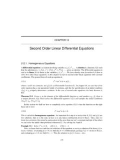
5 = sum of input rates sum of output rates dt By convention, a compartment with no arriving arrowhead has input zero, and a compartment with no exiting arrowhead has output zero. Applying the balance law to Figure 2 gives one differential equation for each of the three compartments x1 , x2 , x3 . 1. x 1 = 0 x1 , 2. 1 1. x 2 = x1 x2 , 2 4. 1 1. x 3 = x2 x3 . 4 6. Recycled Brine Tank Cascade Let brine tanks A, B, C be given of volumes 60, 30, 60, respectively, as in Figure 3. A C. B Figure 3. Three brine tanks in cascade with recycling. Suppose that fluid drains from tank A to B at rate r, drains from tank B to C at rate r, then drains from tank C to A at rate r. The tank volumes remain constant due to constant recycling of fluid. For purposes of illustration, let r = 10. Uniform stirring of each tank is assumed, which implies uniform salt concentration throughout each tank. Let x1 (t), x2 (t), x3 (t) denote the amount of salt at time t in each tank.

6 No salt is lost from the system , due to recycling. Using compartment 524 Systems of Differential Equations analysis, the recycled cascade is modeled by the non-triangular system 1 1. x 1 = x1 + x3 , 6 6. 1 1. x 2 = x1 x2 , 6 3. 1 1. x 3 = x2 x3 . 3 6. The solution is given by the Equations x1 (t) = c1 + (c2 2c3 )e t/3 cos(t/6) + (2c2 + c3 )e t/3 sin(t/6), 1. x2 (t) = c1 + ( 2c2 c3 )e t/3 cos(t/6) + (c2 2c3 )e t/3 sin(t/6), 2. x3 (t) = c1 + (c2 + 3c3 )e t/3 cos(t/6) + ( 3c2 + c3 )e t/3 sin(t/6). At infinity, x1 = x3 = c1 , x2 = c1 /2. The meaning is that the total amount of salt is uniformly distributed in the tanks, in the ratio 2 : 1 : 2. Pond Pollution Consider three ponds connected by streams, as in Figure 4. The first pond has a pollution source, which spreads via the connecting streams to the other ponds. The plan is to determine the amount of pollutant in each pond. 3 2. Figure 4. Three ponds 1, 2, 3. of volumes V1 , V2 , V3 connected f (t) 1 by streams.

7 The pollution source f (t) is in pond 1. Assume the following. Symbol f (t) is the pollutant flow rate into pond 1 (lb/min). Symbols f1 , f2 , f3 denote the pollutant flow rates out of ponds 1, 2, 3, respectively (gal/min). It is assumed that the pollutant is well-mixed in each pond. The three ponds have volumes V1 , V2 , V3 (gal), which remain con- stant. Symbols x1 (t), x2 (t), x3 (t) denote the amount (lbs) of pollutant in ponds 1, 2, 3, respectively. Examples of Systems 525. The pollutant flux is the flow rate times the pollutant concentration, , pond 1 is emptied with flux f1 times x1 (t)/V1 . A compartment analysis is summarized in the following diagram. f (t) f1 x1 /V1. x1 x2. Figure 5. Pond diagram. f3 x3 /V3 The compartment diagram f2 x2 /V2. represents the three-pond x3 pollution problem of Figure 4. The diagram plus compartment analysis gives the following differential Equations . f3 f1. x 1 (t) = x3 (t) x1 (t) + f (t), V3 V1. f1 f2.

8 X 2 (t) = x1 (t) x2 (t), V1 V2. f2 f3. x 3 (t) = x2 (t) x3 (t). V2 V3. For a specific numerical example, take fi /Vi = , 1 i 3, and let f (t) = lb/min for the first 48 hours (2880 minutes), thereafter f (t) = 0. We expect due to uniform mixing that after a long time there will be ( )(2880) = 360 pounds of pollutant uniformly deposited, which is 120 pounds per pond. Initially, x1 (0) = x2 (0) = x3 (0) = 0, if the ponds were pristine. The specialized problem for the first 48 hours is x 1 (t) = x3 (t) x1 (t) + , x 2 (t) = x1 (t) x2 (t), x 3 (t) = x2 (t) x3 (t), x1 (0) = x2 (0) = x3 (0) = 0. The solution to this system is ! !! 3t 2000 125 3 3t 125 3t 125 t x1 (t) = e sin cos + + , 9 2000 3 2000 3 24.. 250 3 3t 3t t x2 (t) = e 2000 sin( )+ , 9 2000 24. ! !! 3t 2000 125 3t 125 3 3t t 125. x3 (t) = e cos + sin + . 3 2000 9 2000 24 3. After 48 hours elapse, the approximate pollutant amounts in pounds are x1 (2880) = , x2 (2880) = , x3 (2880) = It should be remarked that the system above is altered by replacing by zero, in order to predict the state of the ponds after 48 hours.

9 The 526 Systems of Differential Equations corresponding homogeneous system has an equilibrium solution x1 (t) =. x2 (t) = x3 (t) = 120. This constant solution is the limit at infinity of the solution to the homogeneous system , using the initial values x1 (0) . , x2 (0) , x3 (0) Home Heating Consider a typical home with attic, basement and insulated main floor. Attic Main Floor Figure 6. Typical home Basement with attic and basement. The below-grade basement and the attic are un-insulated. Only the main living area is insulated. It is usual to surround the main living area with insulation, but the attic area has walls and ceiling without insulation. The walls and floor in the basement are insulated by earth. The basement ceiling is insulated by air space in the joists, a layer of flooring on the main floor and a layer of drywall in the basement. We will analyze the changing temperatures in the three levels using Newton's cooling law and the variables z(t) = Temperature in the attic, y(t) = Temperature in the main living area, x(t) = Temperature in the basement, t = Time in hours.

10 Initial data. Assume it is winter time and the outside temperature in constantly 35 F during the day. Also assumed is a basement earth temperature of 45 F. Initially, the heat is off for several days. The initial values at noon (t = 0) are then x(0) = 45, y(0) = z(0) = 35. Portable heater. A small electric heater is turned on at noon, with thermostat set for 100 F. When the heater is running, it provides a 20 F. rise per hour, therefore it takes some time to reach 100 F (probably never!). Newton's cooling law Temperature rate = k(Temperature difference). will be applied to five boundary surfaces: (0) the basement walls and floor, (1) the basement ceiling, (2) the main floor walls, (3) the main Examples of Systems 527. floor ceiling, and (4) the attic walls and ceiling. Newton's cooling law gives positive cooling constants k0 , k1 , k2 , k3 , k4 and the Equations x = k0 (45 x) + k1 (y x), y = k1 (x y) + k2 (35 y) + k3 (z y) + 20, z = k3 (y z) + k4 (35 z).