Transcription of The Capital Asset Pricing Model: Theory and Evidence
1 The Capital Asset Pricing Model: Theory and EvidenceEugene F. Fama and Kenneth R. FrenchThe Capital Asset Pricing model (CAPM) of William Sharpe (1964) and JohnLintner (1965) marks the birth of Asset Pricing Theory (resulting in aNobel Prize for Sharpe in 1990). Four decades later, the CAPM is stillwidely used in applications, such as estimating the cost of Capital for firms andevaluating the performance of managed portfolios. It is the centerpiece of MBAinvestment courses. Indeed, it is often the only Asset Pricing model taught in attraction of the CAPM is that it offers powerful and intuitively pleasingpredictions about how to measure risk and the relation between expected returnand risk.
2 Unfortunately, the empirical record of the model is poor poor enoughto invalidate the way it is used in applications. The CAPM s empirical problems mayreflect theoretical failings, the result of many simplifying assumptions. But they mayalso be caused by difficulties in implementing valid tests of the model. For example,the CAPM says that the risk of a stock should be measured relative to a compre-hensive market portfolio that in principle can include not just traded financialassets, but also consumer durables, real estate and human Capital . Even if we takea narrow view of the model and limit its purview to traded financial assets, is it1 Although every Asset Pricing model is a Capital Asset Pricing model, the finance profession reserves theacronym CAPM for the specific model of Sharpe (1964), Lintner (1965) and Black (1972) discussedhere.
3 Thus, throughout the paper we refer to the Sharpe-Lintner-Black model as the F. Fama is Robert R. McCormick Distinguished Service Professor of Finance,Graduate School of Business, University of Chicago, Chicago, Illinois. Kenneth R. French isCarl E. and Catherine M. Heidt Professor of Finance, Tuck School of Business, DartmouthCollege, Hanover, New Hampshire. Their e-mail addresses are and , of Economic Perspectives volume 18, Number 3 Summer 2004 Pages 25 46legitimate to limit further the market portfolio to common stocks (a typicalchoice), or should the market be expanded to include bonds, and otherfinancialassets, perhaps around the world?
4 In the end, we argue that whether the model sproblems reflect weaknesses in the Theory or in its empirical implementation, thefailure of the CAPM in empirical tests implies that most applications of the modelare begin by outlining the logic of the CAPM, focusing on its predictions aboutrisk and expected return. We then review the history of empirical work and what itsays about shortcomings of the CAPM that pose challenges to be explained byalternative Logic of the CAPMThe CAPM builds on the model of portfolio choice developed by HarryMarkowitz (1959). In Markowitz s model, an investor selects a portfolio at timet 1 that produces a stochastic return att.
5 The model assumes investors are riskaverse and, when choosing among portfolios, they care only about the mean andvariance of their one-period investment return. As a result, investors choose mean-variance-efficient portfolios, in the sense that the portfolios 1) minimize thevariance of portfolio return, given expected return, and 2) maximize expectedreturn, given variance. Thus, the Markowitz approach is often called a mean-variance model. The portfolio model provides an algebraic condition on Asset weights in mean-variance-efficient portfolios. The CAPM turns this algebraic statement into a testableprediction about the relation between risk and expected return by identifying aportfolio that must be efficient if Asset prices are to clear the market of all (1964) and Lintner (1965) add two key assumptions to the Markowitzmodel to identify a portfolio that must be mean-variance-efficient.
6 Thefirst assump-tion iscomplete agreement: given market clearing Asset prices att 1, investors agreeon the joint distribution of Asset returns fromt 1tot. And this distribution is thetrue one that is, it is the distribution from which the returns we use to test themodel are drawn. The second assumption is that there isborrowing and lending at arisk-free rate, which is the same for all investors and does not depend on the amountborrowed or 1 describes portfolio opportunities and tells the CAPM story. Thehorizontal axis shows portfolio risk, measured by the standard deviation of portfolioreturn; the vertical axis shows expected return.
7 The curveabc, which is called theminimum variance frontier, traces combinations of expected return and risk forportfolios of risky assets that minimize return variance at different levels of ex-pected return. (These portfolios do not include risk-free borrowing and lending.)The tradeoff between risk and expected return for minimum variance portfolios isapparent. For example, an investor who wants a high expected return, perhaps atpointa, must accept high volatility. At pointT, the investor can have an interme-26 Journal of Economic Perspectivesdiate expected return with lower volatility.
8 If there is no risk-free borrowing orlending, only portfolios abovebalongabcare mean-variance-efficient, since theseportfolios also maximize expected return, given their return risk-free borrowing and lending turns the efficient set into a straightline. Consider a portfolio that invests the proportionxof portfolio funds in arisk-free security and 1 xin some portfoliog. If all funds are invested in therisk-free security that is, they are loaned at the risk-free rate of interest the resultis the pointRfin Figure 1, a portfolio with zero variance and a risk-free rate ofreturn.
9 Combinations of risk-free lending and positive investment ingplot on thestraight line betweenRfandg. Points to the right ofgon the line representborrowing at the risk-free rate, with the proceeds from the borrowing used toincrease investment in portfoliog. In short, portfolios that combine risk-freelending or borrowing with some risky portfoliogplot along a straight line fromRfthroughgin Figure , the return, expected return and standard deviation of return on portfolios of the risk-freeassetfand a risky portfoliogvary withx, the proportion of portfolio funds invested inf,asRp xRf 1 x Rg,E Rp xRf 1 x E Rg , Rp 1 x Rg ,x ,which together imply that the portfolios plot along the line fromRfthroughgin Figure 1 Investment OpportunitiesMinimum variancefrontier for risky assetsgs(R)acbTE(R)
10 RfMean-variance-efficient frontierwith a riskless assetEugene F. Fama and Kenneth R. French27To obtain the mean-variance-efficient portfolios available with risk-free bor-rowing and lending, one swings a line fromRfin Figure 1 up and to the left as faras possible, to the tangency portfolioT. We can then see that all efficient portfoliosare combinations of the risk-free Asset (either risk-free borrowing or lending) anda single risky tangency portfolio,T. This key result is Tobin s (1958) separationtheorem. The punch line of the CAPM is now straightforward. With complete agreementabout distributions of returns, all investors see the same opportunity set (Figure 1),and they combine the same risky tangency portfolioTwith risk-free lending orborrowing.