Transcription of The carbon cycle - ECMWF
1 The carbon cycle in the C-IFS model for atmospheric composition and weather prediction Anna Agusti-Panareda Sebastien Massart, Mark Parrington, Miha Ratzinger, Luke Jones, Michail Diamantakis Gianpaolo Balsamo, Souhail Boussetta Emanuel Dutra, Joaquin Munoz-Sabater, Alessio Bozzo, Robin Hogan, Richard Forbes ( ECMWF ). Frederic Chevallier, Phillippe Peylin, Natasha MacBean, Fabienne Maignan (LSCE). Funded by the European Union Implemented by The carbon cycle Interaction between all the Earth system components carbon reservoirs and their interactions with the atmosphere (focusing on CO2 primarily). Can carbon cycle climate feedbacks improve atmospheric predictive skill? Vegetation, radiative transfer, atmospheric chemistry Atmospheric CO2 and CH4 analysis and forecast (Copernicus Service). Funded by the European Union The 'spheres' of influence Implementedon by the climate system. Source from Institute for Computational Earth System Science(ICESS).
2 The atmospheric reservoir in the fast carbon cycle (annual time-scale). Movement of carbon between land, atmosphere, and oceans: Yellow numbers are natural (balanced fluxes). Red are human contributions (perturbing balance). [Units: in Gigatons of carbon per year]. White numbers: stored carbon [Gigatons of carbon ]. Source: (Diagram adapted from DOE, Biological and Environmental Research Information System.). The atmospheric reservoir: surface observations THE NOAA ANNUAL GREENHOUSE GAS INDEX (AGGI). CO2 growth rate in the atmospheric reservoir The atmospheric concentration growth rate [Gt CO2/year]. In 2015 CO2 increased by 3 ppm ~ 23 GtCO2/year: (droughts associated and fires during el Nino episodes). 15 GtCO2/year ~ 2 ppm/year on average for last 10 years In 1997-1998 el Nino CO2 increased by ppm Source: NOAA-ESRL; Global carbon Budget 2015, LeQuere et al., 2015. Global carbon budget CO2 emissions Partition into resevoirs Source: CDIAC; NOAA-ESRL; Houghton et al 2012; Giglio et al 2013; Joos et al 2013; Khatiwala et al 2013.
3 Le Qu r et al 2015; Global carbon Budget 2015. ANTHROPOGENIC FLUXES. EDGAR inventory of anthropogenic emissions (excluding land-use change). Source: EDGAR database Source: Global carbon Budget 2015; CDIAC. CO2 emissions: land-use change CO2 emissions: land-use change by burning biomass GFAS daily fire product available 1 day behind real time GFAS CO2 emissions over Indonesia (Sep-Oct 2015): Fires contribute to el Nino signal in the atmospheric CO2 growth rate The ocean reservoir in the carbon cycle Solubility pump (inorganic carbon ). Ocean circulation (long timescales). Biological pump (organic carbon ). Wikipedia: Hannes Grobe 21:52, 12 August 2006 (UTC), Alfred Wegener Institute for Polar and Marine Research, Bremerhaven, Germany The CO2 ocean-atmosphere fluxes Climatology of monthly mean ocean fluxes from Takahashi et al. (2009) used in C-IFS. Observations of pCO2 at the surface of the ocean and in the atmosphere with transfer coefficients based on turbulent exchange.
4 Regions of sources and sinks associated with upwelling and downwelling regions Takahashi et al. (2009). The terrestrial CO2 fluxes Strong link with water and energy fluxes Jung et al. (2011). Terrestrial carbon flux : Exchange between the biosphere and the atmosphere Atmospheric CO2 sink (Gross Primary Production): Photosynthesis (plants). CO2 + H2O + energy CH2O + O2. Atmospheric CO2 source (Ecosystem Respiration): Respiration CH2O + O2 CO2 + H2O + energy (plants, animals) CH2O CH4 + energy in anoxic conditions + decomposition of organic carbon in soil by microbes Illustration adapted from Sellers et al., 1992 Credit: Raphael Gabriel Modelling CO2 uptake by plants (GPP) in C-IFS. Environmental factors: 1. rs . gs - Temperature - PAR (solar radiation). An - Soil moisture gs - Atm. wv deficit (Cs Ci ) - Atm. CO2. Biological factors: - Mesophyll conductance + Soil moisture stress function CTESSEL parameterisation based on ISBA-Ags Cs Ci f ( Ds , rm ) Jacobs (1994), Calvet et al.
5 , 1998,2000, Lafont et al. 2012, Cs 340 ppm Boussetta et al. (2013). Modelling CO2 uptake by plants (GPP) in C-IFS. LEAF STOMATA CANOPY MODEL FLUXES. An Anc gs gc GPP. Upscaling to canopy Upscaling to model grid point with with LAI climatology vegetation dominant type/cover from MODIS. CTESSEL parameterisation based on ISBA-Ags Jacobs (1994), Calvet et al., 1998,2000, Lafont et al. 2012, Boussetta et al. (2013). Modelling soil respiration ( (Tsoil 25)) .Z snow ( (Tsoil 25)). Rsoil R Q 0 10 fsm Rsoil R e 0 10Q sm f Environmental factors: Temperature Q10 dependance on Temperature regime 6. Soil moisture Snow depth 5. 4. Biological factors: 3. Q10. 2. Organic carbon in soil 1. and microbial activity (R0 parameter) Including a snow 0. 0 10 20 30 40 50 60. attenuation effect on the T [oC]. soil CO2 emission Including a temeperature dependancy on the Q10 parameter (McGuire et al., 1992). Slide 16.
6 Boussetta et al. (2013). Evaluation of CO2 ecosystem fluxes from CTESSEL in IFS. Example of NEE (micro moles /m2/s) predicted over the site Fi-Hyy (FINLAND) by CTESSEL (black line) and CASA-GFED3 (green-line) compared to FLUXNET observations Scheme NEE rmse NEE bias NEE corr CTESSEL CASA Boussetta et al. (2013) Slide 17. Modelling atmospheric CO2 in C-IFS. Synoptic variability of NEE is important for the CO2. synoptic variability in the BL. In the warm sectors of low pressure systems: synergy between advection and CO2 ecosystem fluxes: GOSAT view cloudy reduction of CO2 uptake More CO2 Enhanced atmospheric CO2 anomaly warm increase in respiration Agusti-Panareda et al. ACP 2014. Modelling atmospheric CO2 in C-IFS. CO2 surface fluxes & column-averaged dry-air mole fraction of CO2 [ppm]. Transport IFS model Fluxes Vegetation (CTESSEL model). Source Sink Fires (GFAS). Ocean (Takahashi et al 2009).
7 Source Sink GOSAT view Anthropogenic (EDGAR ). Symbol size reflects the relative flux intensity (Note that fires have been re-scaled by a factor of 10). Agusti-Panareda et al. ACP 2014. GOSAT. GOSAT analysis analysis (28 November 2014 14. November 2014 14 December December2014). 2014). Model - TCCON obs Analysis - TCCON obs Analysis departure (o-a) No or few GOSAT data to constrain the analysis in In ppm for GOSAT data these regions Massart et al. ACP 2015. Correcting atmospheric CO2 biases with Biogenic Flux Adjustment Scheme (BFAS). ARCHIVED DATA. CAMS CO2 modelling (IFS). EPS FORECAST/HINDCAST. MODELLED. FLUXES. CAMS CO2 FC. CO2 SURFACE FLUXES. BFAS. CTESSEL model Prescribed CTESSEL Compares budgets Anthropogenic BUDGET emissions Re-scaling maps for Adjusted Ocean biogenic fluxes Net Ecosystem sources/sinks from CTESSEL Fluxes OPTIMIZED Fire emissions FLUXES. MACC (LSCE). TRANSPORT.
8 REFERENCE Improved BUDGET atmospheric CO2 forecast Agusti-Panareda et al et al. ACP 2016. Biogenic Flux Adjustment Scheme: Improving the total column CO2. Total column mean TCCON Observations Atmospheric CO2 simulations with optimized fluxes climatology of optimized fluxes Modelled NEE. 2010 Modelled NEE + BFAS. Biogenic Flux Adjustment Scheme: Improving CO2 synoptic variability March 2010. NOAA/ESRL tall tower Observations Atmospheric CO2 simulations with optimized fluxes climatology of optimized fluxes Modelled NEE. Modelled NEE + BFAS. [ppm]. [ppm]. CO2 Ecosystem Flux Adjustment factors: what can we learn to improve the model? Crops Reco factor GPP factor Re-tune the reference respiration for crops Distinction between C3 and C4 crops necessary Revision of vegetation types: A new subtype of interrupted forest for BFAS (tropical savanna). Agusti-Panareda et al et al. ACP 2016. Feedbacks of carbon cycle to NWP: - Improvement in representation of vegetation: photosynthesis, phenology, albedo Jarvis Vs photosynthesis-based evapotranspiration (offline run).
9 HTESSEL CTESSEL. H. Surface sensible heat flux (W/m2) compared with flux-tower observations over Fr-LBr for HTESSEL (left panel) and CTESSEL (right panel). LE. Surface laten heat flux (W/m2) compared with flux-tower observations over Fr-LBr for HTESSEL (left panel) and CTESSEL (right panel). CTESSEL improves the LE/H simulations (Photosynthesis-based vs Jarvis approach). Slide 26. LE/H: When good is not enough? (Interaction with the atmosphere). 2m T Error differences from the CTL 2m Rh Error differences from the CTL. Having better LE/H heat flux from the surface does not always lead to a better atmospheric prediction interaction with other processes and compensating errors? S. Boussetta Slide 27. Modelling stomatal conductance (empirical vs mechanistic approaches): . E (qa qsat ). rc ra The Jarvis (statistical) approach The mechanistic approach CHTESSEL in IFS (operational). CTESSEL in IFS.
10 Rc f (rcc ).. rcc (Cs Ci ). Aspects Jarvis model CTESSEL model An Simplicity/robustness Yes No Copernicus atmospheric CO2. Coupling with carbon cycle No Yes forecast/analysis & ecosystem CO2 flux Feedbacks on vegetation No Yes Use carbon observations LAI LAI, SIF, GPP, atmospheric CO2 for mass balance Feedbacks from vegetation: Impact of assimilating LAI on 2m temperature -3 -1 0 1 3. NRT_LAI_ALB FCLIM: November 2010. Severe drought in the Horn of Africa Red Warming T2m -3 -1 0 1 3. Err T2m 29. S. Boussetta Feedbacks from vegetation: Impact of assimilating LAI on albedo Blue Better forecast Blue Better forecast Err T2m Red Worse forecast Err RH2m Red Worse forecast Reduction of cold/moist bias in 3-day FC over northern Europe in March 2015. S. Boussetta Slide 30. Impact of dynamic vegetation on monthly forecast in semi-arid regions Improved skill of monthly forecast 2m-T with soil moisture Hot-spots of NEE and GPP variability and dynamic phenology compared to fc with climatologies Koster and Walker (2015) Jung et al.