Transcription of The Level Set Method - MIT Mathematics
1 The Level Set MethodMIT / / Methods for Partial Differential EquationsPer-Olof Persson 8, 2005 Evolving Curves and Surfaces Propagate curve according to speed functionv=Fn Fdepends on space, time, and the curve itself Surfaces in three dimensionsFGeometry RepresentationsExplicit Geometry Parameterized boundaries(x, y) = (x(s), y(s))Implicit Geometry Boundaries given by zero Level set (x, y) = 0 (x, y)<0 (x, y)>0 Explicit Techniques Simple approach: Represent curve explicitly by nodesx(i)and lines Propagate curve by solving ODEsdx(i)dt=v(x(i), t),x(i)(0) =x(i)0, Normal vector, curvature, etc by difference approximations, :dx(i)ds x(i+1) x(i 1)2 s MATLAB DemoExplicit Techniques - Drawbacks Node redistribution required, introduces errors No entropy solution, sharp corners handled incorrectly Need special treatment for topology changes Stability constraints for curvature dependent speed functionsNode distributionSharp cornersTopology changesThe Level Set Method Implicit geometries, evolve interface by solving PDEs Invented in 1988 by Osher and Sethian: Stanley Osher and James A.
2 Sethian. Fronts propagating withcurvature-dependent speed: algorithms based on Comput. Phys., 79(1):12 49, 1988. Two good introductory books: James A. set methods and fast marching University Press, Cambridge, second edition, 1999. Stanley Osher and Ronald set methods and dynamicimplicit surfaces. Springer-Verlag, New York, Geometries Represent curve by zero Level set of a function, (x) = 0 Special case:Signed distance function: | |= 1 | (x)|gives (shortest) distance fromxto curve >0 <0 Discretized Implicit Geometries Discretize implicit function onbackground grid Obtain (x)for generalxby interpolationCartesianQuadtree/OctreeGeo metric Variables Normal vectorn(without assuming distance function):n= | | Curvature (in two dimensions): = | |= xx 2y 2 y x xy+ yy 2x( 2x+ 2y)3/2. Write material parameters, etc, in terms of : (x) = 1+ ( 2 1) ( (x))Smooth Heaviside function over a few grid Level Set Equation Solve convection equation to propagate = 0by velocitiesv t+v = 0.
3 Forv=Fn, usen= /| |and =| |2to obtain theLevel Set Equation t+F| |= 0. Nonlinear, hyperbolic equation (Hamilton-Jacobi).Discretization Use upwinded finite difference approximations for convection For the Level set equation t+F| |= 0: n+1ijk= nijk+ t1 max(F,0) +ijk+ min(F,0) ijk ,where +ijk= max(D x nijk,0)2+ min(D+x nijk,0)2+max(D y nijk,0)2+ min(D+y nijk,0)2+max(D z nijk,0)2+ min(D+z nijk,0)2 1/2,Discretizationand ijk= min(D x nijk,0)2+ max(D+x nijk,0)2+min(D y nijk,0)2+ max(D+y nijk,0)2+min(D z nijk,0)2+ max(D+z nijk,0)2 1/2. D xbackward difference operator in thex-direction, etc For curvature dependent part ofF, use central differences Higher order schemes available MATLAB DemoReinitialization Large variations in for general speed functionsF Poor accuracy and performance, need smaller timesteps for stability Reinitializeby finding new with same zero Level set but| |= 1 Different approaches:1.
4 Integrate thereinitialization equationfor a few time steps t+ sign( )(| | 1) = 02. Compute distances from = 0explicitly for nodes close to boundary,use Fast Marching Method for remaining nodesThe Boundary Value Formulation ForF >0, formulate evolution by an arrival functionT T(x)gives time to reachxfrom initial time * rate = distance gives theEikonal equation:| T|F= 1, T= 0on . Special case:F= 1gives distance functionsyxT(x,y)The Fast Marching Method Discretize the Eikonal equation| T|F= 1by max(D xijkT,0)2+ min(D+xijkT,0)2+ max(D yijkT,0)2+ min(D+yijkT,0)2+ max(D zijkT,0)2+ min(D+zijkT,0)2 1/2=1 Fijkor max(D xijkT, D+xijkT,0)2+ max(D yijkT, D+yijkT,0)2+ max(D zijkT, D+zijkT,0)2 1/2=1 FijkThe Fast Marching Method Use the fact that the front propagates outward Tag known values and update neighboringTvalues (using the differenceapproximation) Pick unknown with smallestT(will not be affected by other unknowns) Update new neighbors and repeat until all nodes are known Store unknowns in priority queue,O(nlogn)performance fornnodeswith heap implementationApplicationsFirst arrivals and shortest geodesic pathsVisibility around obstaclesStructural Vibration Control Consider eigenvalue problem u= (x)u,x u= 0,x.
5 With (x) = 1forx / S 2forx S. Solve the optimizationminS 1or 2subject tokSk=K. \S, 1S, 2 Structural Vibration Control Level set formulation by Osher and Santosa: Finite difference approximations for Laplacian Sparse eigenvalue solver for solutions i, ui Calculate descent direction = v(x)| |withv(x)from shapesensitivity analysis Find Lagrange multiplier for area constraint using Newton s Method Represent interface implicitly, propagate using Level set methodStress Driven Rearrangement Instabilities Epitaxial growth of InAs on a GaAs substrate, stress from misfit in lattices Quasi-static interface evolution, descent direction for elasticenergy andsurface energy +F(x)| |= 0,withF(x) = (x) (x) Level set formulation by Persson, finite elements for the elasticityElectron micrograph of defect-free InAs quantum dotsStress Driven Rearrangement InstabilitiesInitial ConfigurationFinal Configuration, = Driven Rearrangement InstabilitiesInitial ConfigurationFinal Configuration, = Driven Rearrangement InstabilitiesInitial ConfigurationFinal Configuration, =