The mathematics of PDEs and the wave equation

1 The mathematics of PDEs and the wave equationMichael P. Lamoureux University of CalgarySeismic Imaging Summer SchoolAugust 7 11, 2006, CalgaryAbstractAbstract: We look at the mathematical theory of partial differential equations asapplied to the wave equation . In particular, we examine questions about existence anduniqueness of solutions, and various solution techniques. Supported by NSERC, MITACS and the POTSI and CREWES 2006. All rights Lecture One: Introduction to PDEs equations from physics Deriving the 1D wave equation One way wave equations Solution via characteristic curves Solution via separation of variables Helmholtz equation Classification of second order, linear PDEs Hyperbolic equations and the wave equation2. Lecture Two: Solutions to PDEs with boundary conditions and initial conditions Boundary and initial conditions Cauchy, Dirichlet, and Neumann conditions Well-posed problems Existence and uniqueness theorems D Alembert s solution to the 1D wave equation Solution to the n-dimensional wave equation Huygens principle Energy and uniqueness of solutions3.

2 Lecture Three: Inhomogeneous solutions - source terms Particular solutions and boundary, initial conditions Solution via variation of parameters Fundamental solutions Green s functions, Green s theorem Why the convolution with fundamental solutions? The Fourier transform and solutions Analyticity and avoiding zeros Spatial Fourier transforms Radon transform Things we haven t covered21 Lecture One: Introduction to PDEsA partial differential equation is simply an equation that involves both a function and itspartial derivatives. In these lectures, we are mainly concerned with techniques to find asolution to a given partial differential equation , and to ensure good properties to that solu-tion. That is, we are interested in the mathematical theory of the existence, uniqueness, andstability of solutions to certain PDEs, in particular the wave equation in its various of the equations of interest arise from physics, and we will usex, y, zas the usualspatial variables, andtfor the the time variable.

3 Various physical quantities will be measuredby some functionu=u(x, y, z, t) which could depend on all three spatial variable and time,or some subset. The partial derivatives ofuwill be denoted with the following condensednotationux= u x, uxx= 2u x2, ut= u t, uxt= 2u x tand so Laplace operator is the most physically important differential operator,which is given by 2= 2 x2+ 2 y2+ 2 equations from physicsSome typical partial differential equations that arise in physics are as sequation 2u= 0which is satisfied by the temperatureu=u(x, y, z) in a solid body that is in thermalequilibrium, or by the electrostatic potentialu=u(x, y, z) in a region without heat equationut=k 2uwhich is satisfied by the temperatureu=u(x, y, z, t) of a physical object which conductsheat, wherekis a parameter depending on the conductivity of the waveequationutt=c2 2uwhich models the vibrations of a string in one dimensionu=u(x, t), the vibrations of a thinmembrane in two dimensionsu=u(x, y, t)

4 Or the pressure vibrations of an acoustic wavein airu=u(x, y, z, t). The constantcgives the speed of propagation for the related to the 1D wave equation is the fourth order2 PDE for a vibrating beam,utt= c2uxxxx1We assume enough continuity that the order of differentiation is unimportant. This is true anyway in adistributional sense, but that is more detail than we need to order of a PDE is just the highest order of derivative that appears in the here the constantc2is the ratio of the rigidity to density of the beam. An interestingnonlinear3version of the wave equation is the Korteweg-de Vries equationut+cuux+uxxx= 0which is a third order equation , and represents the motion of waves in shallow water, as wellas solitons in fibre optic are many more examples. It is worthwhile pointing out that while these equationscan be derived from a careful understanding of the physics of each problem, some intuitiveideas can help guide us.

5 For instance, the Laplacian 2u= 2u x2+ 2u y2+ 2u z2can be understood as a measure of how much a functionu=u(x, y, z) differs at one point(x, y, z) from its neighbouring points. So, if 2uis zero at some point (x, y, z), thenu(x, y, z)is equal to the average value ofuat the neighbouring points, say in a small disk around(x, y, z). If 2uis positive at that point (x, y, z), thenu(x, y, z) is smaller than the averagevalue ofuat the neighbouring points. And if 2u(x, y, z) is negative, thenu(x, y, z) is largerthat the average value ofuat the neighbouring , Laplace s equation 2u= 0represents temperature equilibrium, because if the temperatureu=u(x, y, z) at a particularpoint (x, y, z) is equal to the average temperature of the neighbouring points, no heat willflow. The heat equationut=k 2uis simply a statement of Newton s law of cooling, that the rate of change of temperature isproportional to the temperature difference (in this case, the difference between temperatureat point (x, y, z) and the average of its neighbours).

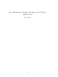
6 The wave equationutt=c2 2is simply Newton s second law (F=ma) and Hooke s law (F=k x) combined, so thataccelerationuttis proportional to the relative displacement ofu(x, y, z) compared to itsneighbours. The constantc2comes from mass density and elasticity, as expected in Newton sand Hooke s Deriving the 1D wave equationMost of you have seen the derivation of the 1D wave equation from Newton s and Hooke s key notion is that the restoring force due to tension on the string will be proportional3 Nonlinear because we seeumultiplied byuxin the the curvature at the point, as indicated in the figure. Then mass times acceleration uttshould equal that force,kuxx. Thusutt=c2uxxwherec= k/ turns out to be the velocity of 1: The restoring forces on a vibrating string, proportional to s do it again, from an action (x, t) denote the deplacement of a string from the neutral positionu 0.

7 Themass density of the string is given by = (x) and the elasticity given byk=k(x). Inparicular, in this derivation we do not assuming the the string is uniform. Consider a shortpiece of string, in the interval [x, x+ x]. Its mass with be (x) x, its velocityut(x, t), andthus its kinetic energy, one half mass times velocity squared, is K=12 (ut)2 total kinetic energy for the string is given by an integral,K=12 L0 (ut) Hooke s law, the potential energy for a string is (k/2)y2, whereyis the length of thespring. For the stretched string, the length of the string is given by arclengthds= 1 +u2xdxand so we expect a potential energy of the formP= L0k2(1 +u2x) action for a given functionuis defined as the integral over time of the difference ofthese two energies, soL(u) =12 T0 L0 (ut)2 k [1 + (ux)2]dx one doesn t really need to be in there, but it doesn t matter for a potential times a perturbationh=h(x, t) to the functionugives a new actionL(u+ h) =L(u) + T0 L0 ut ht k uxhxdx dt+ higher order in.

8 The principle of least action says that in order foruto be a physical solution, the first orderterm should vanish for any perturbationh. Integration by parts (intfor the first term, inxfor the second term, and assuminghis zero on the boundary) gives0 = T0 L0( utt+k uxx+kx ux) h dx this integral is zero for all choices ofh, the first factor in the integral must be zero,and we obtain the wave equation for an inhomogeneous medium, utt=k uxx+kx the elasticitykis constant, this reduces to usual two term wave equationutt=c2uxxwhere the velocityc= k/ varies for changing One way wave equationsIn the one dimensional wave equation , whencis a constant, it is interesting to observe thatthe wave operator can be factored as follows( t2 c2 x2)=( t c x)( t+c x).We could then look for solutions that satisfy the individual first order equationsut cux= 0 orut+cux= are one way wave equations , and the general solution to the two way equation couldbe done by forming linear combinations of such solutions.

9 The solutions of the one waveequations will be discussed in the next section, using characteristic linesct x= constant,ct+x= way to solve this would be to make a change of coordintates, =x ct, =x+ctand observe the second order equation becomesu = 0which is easily higher dimensions, one could hope to factor the second order wave equation in theform( t2 c2 2)=( t cD)( t+cD),whereDis some first order partial differential operator (independent oft) which satisfiesD2= luck solving this operatorDis called the Dirac operator; findingparticular Dirac operators is a major intellectual achievement of modern mathematics andphysics. The Atiyah-Singer index theorem is a deep result connecting the Dirac operatorwith the geometry of Solution via characteristic curvesOne method of solution is so simple that it is often overlooked. Consider the first orderlinear equation in two variables,ut+cux= 0,which is an example of a one-way wave equation .

10 To solve this, we notice that along the linex ct= constantkin thex, tplane, that any solutionu(x, y) will be constant. For if wetake the derivative ofualong the linex=ct+k, we have,ddtu(ct+k, t) =cux+ut= 0,souis constant on this line, and only depends on the choice of parameterk. Call thisfunctional dependencef(k) and thus we may setu(x, t) =f(k) =f(x ct).That is, given any differentiable functionfon the real line, we obtain a solutionu(x, t) =f(x ct)and all solutions are of this form. Note this solution represents simply the waveformf(x)moving along to the right at is a question of initial conditions and boundary values. In fact,if we are given the initial values foru=u(x,0) then this determinesf, sinceu(x,0) =f(x c0) =f(x). That is, the initial values forudetermine the functionf, and the functionfdeterminesueverywhere on the plane by following the characteristic note in passing that in the usual (two-way) wave equation in three dimensions,utt=c2 2u,5 You might ask yourself, why notD= ?