The Numerical Method of Lines for Partial Differential ...

1 1 The Numerical Method of Lines for PartialDifferential Equationsby Michael B. Cutlip, University of Connecticut andMordechai Shacham, Ben-Gurion University of the NegevThe Method of Lines is a general technique for solving Partial Differential equations (PDEs) by typically using finite difference relationships for the spatial derivatives andordinary Differential equations for the time derivative. William E. Schiesser at LehighUniversity has been a major proponent of the Numerical Method of Lines , Thissolution approach can be very useful with undergraduates when this technique isimplemented in conjunction with a convenient ODE solver package such Problem in Unsteady-State Heat Transfer3 This approach can be illustrated by considering a problem in unsteady-state heatconduction in a one-dimensional slab with one face insulated and constant thermalconductivity as discussed by heat transfer in a slab in the x direction is described by the partialdifferential equation22xTtT = (1)where T is the temperature in K, t is the time in s, and is the thermal diffusivity in m2/sgiven by k/ cp.

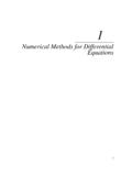
2 In this treatment, the thermal conductivity k in W/m K, the density inkg/m3, and the heat capacity cp in J/kg K are all considered to be that a slab of material with a thickness m is supported on anonconducting insulation. This slab is shown in Figure 1. For a Numerical problemsolution, the slab is divided into N sections with N + 1 node points. The slab is initially at auniform temperature of 100 C. This gives the initial condition that all the internal nodetemperatures are known at time t = = 100 for n = 2 .. (N + 1) at t = 0(2) 1 Schiesser, W. E. The Numerical Method of Lines , San Diego, CA: Academic Press, POLYMATH is a Numerical analysis package for IBM-compatible personal computers that isavailable through the CACHE Corporation.

3 Information can be found at This problem is adapted in part from Cutlip, M. B., and M. Shacham Problem Solving inChemical Engineering with Numerical methods , Upper Saddle River, NJ: Prentice Hall, Geankoplis, C. J. Transport Processes and Unit Operations, 3rd ed. Englewood Cliffs,NJ: Prentice Hall, 1 - Unsteady-State Heat Conduction in a One-dimensional SlabIf at time zero the exposed surface is suddenly held constant at a temperature of0 C, this gives the boundary condition at node 1:T1 = 0 for t 0(3)The other boundary condition is that the insulated boundary at node N + 1 allowsno heat conduction. Thus01= +xTN for t 0(4)Note that this problem is equivalent to having a slab of twice the thickness exposed to theinitial temperature on both (a) - Numerically solve Equation (1) with the initial and boundaryconditions of (2), (3), and (4) for the case where = 2 10-5 m2/s and the slabsurface is held constant at T1 = 0 C.

4 This solution should utilize the numericalmethod of Lines with N = 10 sections. Plot the temperatures T2, T3, T4, and T5 asfunctions of time to 6000 this problem with N = 10 sections of length x = m, Equation (1) can berewritten using a central difference formula for the second derivative as()1122)( ++ = nnnnTTTxtT for (2 n 10)(5)The boundary condition represented by Equation (4) can be written using a second-orderbackward finite difference as02439101111= + = xTTTtT(6)that can be solved for T11 to yield3491011 TTT =(7)3 The problem then requires the solution of equations (3), (5), and (7) whichresults in nine simultaneous ordinary Differential equations and two explicit algebraicequation for the 11 temperatures at the various nodes.

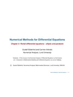
5 This set of equations can be enteredinto the POLYMATH Simultaneous Differential Equation Solver or some other ODEsolver. The resulting equation set for POLYMATH isEquations:d(T2)/d(t)=alpha/deltax^2*(T 3-2*T2+T1)d(T3)/d(t)=alpha/deltax^2*(T4- 2*T3+T2)d(T4)/d(t)=alpha/deltax^2*(T5-2* T4+T3)d(T5)/d(t)=alpha/deltax^2*(T6-2*T5 +T4)d(T6)/d(t)=alpha/deltax^2*(T7-2*T6+T 5)d(T7)/d(t)=alpha/deltax^2*(T8-2*T7+T6) d(T8)/d(t)=alpha/deltax^2*(T9-2*T8+T7)d( T9)/d(t)=alpha/deltax^2*(T10-2*T9+T8)d(T 10)/d(t)=alpha/deltax^2*(T11-2*T10+T9)al pha= (4*T10-T9)/3deltax=.10 The initial condition for each of the T s is 100 and the independent variable t variesfrom 0 to 6000. The plots of the temperatures in the first four sections, node points 2.

6 5, are shown in Figure 2. The transients in temperatures show an approach to steady Numerical results are compared to the hand calculations of a finite difference solutionby Geankoplis4 (pp. 471 3) at the time of 6000 s in Table 1. These results indicate thatthere is general agreement regarding the problem solution, but differences between thetemperatures at corresponding nodes increase as the insulated boundary of the slab 2 Temperature Profiles for Unsteady-state Heat Conduction in aOne-dimensional Slab4 Table 1 Results for Unsteady-state Heat Transfer in a One-dimensionalSlab at t = 6000 sGeankoplis4 Numerical Method of Lines x = = 5 x = mN = 10 x = mN = 20 x = mN = 30 Distancefrom SlabSurface in (b) - Repeat Problem (a) with 20 sections and compare results with part(a).

7 The validity of the Numerical solution can be investigated by doubling the numberof sections for the NMOL solution. This involves adding an additional 10 equations givenby the relationship in Equation (5), modifying Equation (7) to calculate T21, and halving x. The results for these changes in the POLYMATH equation set are also summarized inTable 1 as are similar results for 30 sections. Here the Numerical solutions are similar tothe previous solution in part (a) as the temperature profiles are virtually unchanged as thenumber of section is (c) - Repeat parts (a) and (b) for the case where heat convection is presentat the slab surface. The heat transfer coefficient is h = W/m 2 K, and thethermal conductivity is k = W/m convection is considered as the only mode of heat transfer to the surface ofthe slab, an energy balance can be made at the interface that relates the energy input byconvection to the energy output by conduction.

8 Thus at any time for transport normal tothe slab surface in the x direction010)(= = xxTkTTh(8)where h is the convective heat transfer coefficient in W/m2 K and T0 is the preceding energy balance at the slab surface can be used to determine arelationship between the slab surface temperature T1, the ambient temperature T0, and thetemperatures at internal node points. In this case, the second-order forward differenceequation for the first derivative can be applied at the surface()xTTTxTx + = =2341230(9)5and can be substituted into Equation (8) to yield()xTTTkTTh + = 234)(12310(10)The preceding equation can be solved for T1 to givexhkkTkTxhTT ++ =23422301(11)and the above equation can be used to calculate T1 during the NMOL resulting equation set for POLYMATH for x = m for N = 10 isEquations.

9 D(T2)/d(t)=alpha/deltax^2*(T3-2*T2+T1)d( T3)/d(t)=alpha/deltax^2*(T4-2*T3+T2)d(T4 )/d(t)=alpha/deltax^2*(T5-2*T4+T3)d(T5)/ d(t)=alpha/deltax^2*(T6-2*T5+T4)d(T6)/d( t)=alpha/deltax^2*(T7-2*T6+T5)d(T7)/d(t) =alpha/deltax^2*(T8-2*T7+T6)d(T8)/d(t)=a lpha/deltax^2*(T9-2*T8+T7)d(T9)/d(t)=alp ha/deltax^2*(T10-2*T9+T8)d(T10)/d(t)=alp ha/deltax^2*(T11-2*T10+T9)alpha= (4*T10-T9)/3h= (2*h*T0*deltax-k*T3+4*k*T2)/(3*k+2*h*del tax)The preceding equation set can be integrated to any time t with POLYMATH oranother ODE solver. The results at t = 1500 s are summarized in Table 2 Results for Unsteady-state Heat Transfer with Convection in aOne-dimensional Slab at t = 1500 sGeankoplis4 Numerical Method of Lines x = = 5 x = mN = 10 x = mN = 20 x = mN = 30 Distancefrom SlabSurface in is reasonable agreement between the various NMOL results as the numberof sections (smaller x) is increased.

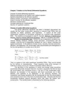
10 The slower response of the temperatures within the6slab due to the additional convective resistance to heat transfer is evident when thetemperatures are compared to those presented in Table 1. Selected temperatures arepresented in Figure 3 for the same locations and at the same scale as Figure 2. The delaysin the responses of the various temperatures are quite 3 Temperature Profiles for Unsteady-state Heat Transfer with Convectionin a One-dimensional SlabProblem ExtensionsThere are a number of extensions to this problem that can be solved with theNumerical Method of Lines . The thermal conductivity of the solid could vary with thelocal temperature. There could be an initial temperature profile in the solid.