Transcription of The Scientist and Engineer's Guide to Digital Signal ...
1 581 CHAPTER32 The Laplace TransformThe two main techniques in Signal processing , convolution and Fourier analysis, teach that alinear system can be completely understood from its impulse or frequency response. This is avery generalized approach, since the impulse and frequency responses can be of nearly any shapeor form. In fact, it is too general for many applications in science and engineering. Many of theparameters in our universe interact through differential equations. For example, the voltageacross an inductor is proportional to the derivative of the current through the device. Likewise,the force applied to a mass is proportional to the derivative of its velocity.
2 Physics is filled withthese kinds of relations. The frequency and impulse responses of these systems cannot bearbitrary, but must be consistent with the solution of these differential equations. This means thattheir impulse responses can only consist of exponentials and sinusoids. The Laplace transformis a technique for analyzing these special systems when the signals are continuous. The z-transform is a similar technique used in the discrete Nature of the s-DomainThe Laplace transform is a well established mathematical technique for solvingdifferential equations. It is named in honor of the great French mathematician,Pierre Simon De Laplace (1749-1827).
3 Like all transforms, the Laplacetransform changes one Signal into another according to some fixed set of rulesor equations. As illustrated in Fig. 32-1, the Laplace transform changes asignal in the time domain into a Signal in the s-domain, also called the s-plane. The time domain Signal is continuous, extends to both positive andnegative infinity, and may be either periodic or aperiodic. The Laplacetransform allows the time domain to be complex; however, this is seldomneeded in Signal processing . In this discussion, and nearly all practicalapplications, the time domain Signal is completely shown in Fig.
4 32-1, the s-domain is a complex plane, , there are realnumbers along the horizontal axis and imaginary numbers along the verticalaxis. The distance along the real axis is expressed by the variable, F, a lowerThe Scientist and Engineer's Guide to Digital Signal Processing582X(T)'m4&4x(t)e&jTtdtX(F,T)' m4&4[x(t)e&Ft]e&jTtdtcase Greek sigma. Likewise, the imaginary axis uses the variable, T, thenatural frequency. This coordinate system allows the location of any point tobe specified by providing values for F and T. Using complex notation, eachlocation is represented by the complex variable, s, where: . Just ass'F%jTwith the Fourier transform, signals in the s-domain are represented by capitalletters.
5 For example, a time domain Signal , , is transformed into an s-x(t)domain Signal , , or alternatively, . The s-plane is continuous, andX(s)X(F,T)extends to infinity in all four directions. In addition to having a location defined by a complex number, each point in thes-domain has a value that is a complex number. In other words, each locationin the s-plane has a real part and an imaginary part. As with all complexnumbers, the real & imaginary parts can alternatively be expressed as themagnitude & as the Fourier transform analyzes signals in terms of sinusoids, the Laplacetransform analyzes signals in terms of sinusoids and exponentials.
6 From amathematical standpoint, this makes the Fourier transform a subset of the moreelaborate Laplace transform. Figure 32-1 shows a graphical description of howthe s-domain is related to the time domain. To find the values along a verticalline in the s-plane (the values at a particular F), the time domain Signal is firstmultiplied by the exponential curve: . The left half of the s-planee&Ftmultiplies the time domain with exponentials that increase with time (),F<0while in the right half the exponentials decrease with time (). Next, takeF>0the complex Fourier transform of the exponentially weighted Signal . Theresulting spectrum is placed along a vertical line in the s-plane, with the tophalf of the s-plane containing the positive frequencies and the bottom halfcontaining the negative frequencies.
7 Take special note that the values on they-axis of the s-plane () are exactly equal to the Fourier transform of theF'0time domain Signal . As discussed in the last chapter, the complex Fourier Transform is given by:This can be expanded into the Laplace transform by first multiplying the timedomain Signal by the exponential term:While this is not the simplest form of the Laplace transform, it is probablythe best description of the strategy and operation of the technique. ToChapter 32- The Laplace Transform583 Real axis (F) (t)X(s)F = -3F = -2F = -1F = 0F = 1F = 2F = 3spectrumfor F = 3 Imaginary axis (jT)AmplitudeSTEP 4 Arrange each spectrum along avertical line in the s-plane.
8 Thepositive frequencies are in theupper half of the s-plane while thenegative frequencies are in thelower [x(t)e&Ft]e&jTtdtSTEP 2 Multiply the time domain Signal byan infinite number of exponentialcurves, each with a different decayconstant, F. That is, calculate thesignal: for each value of Fx(t)e&Ftfrom negative to positive 1 Start with the time domain signalcalled x(t)STEP 3 Take the complex Fourier Transformof each exponentially weighted timedomain Signal . That is, calculate:for each value of F from negative topositive 32-1 The Laplace transform. The Laplace transform converts a Signal in the time domain, , into a Signal in the s-domain,x(t). The values along each vertical line in the s-domain can be found by multiplying the time domain signalX(s)orX(F,T)by an exponential curve with a decay constant F, and taking the complex Fourier transform.
9 When the time domain isentirely real, the upper half of the s-plane is a mirror image of the lower half. The Scientist and Engineer's Guide to Digital Signal Processing584X(F,T)'m4&4x(t)e&(F%jT)tdtE QUATION 32-1 The Laplace transform. This equationdefines how a time domain Signal , , isx(t)related to an s-domain Signal , . The s-X(s)domain variables, s, and , are ()While the time domain may be complex, it isusually (s)'m4&4x(t)e&stdtplace the equation in a shorter form, the two exponential terms can becombined:Finally, the location in the complex plane can be represented by the complexvariable, s, where . This allows the equation to be reduced to an evens'F%jTmore compact expression:This is the final form of the Laplace transform, one of the mostimportant equations in Signal processing and electronics.
10 Pay specialattention to the term: , called a complex exponential. As shown by thee&stabove derivation, complex exponentials are a compact way of representing bothsinusoids and exponentials in a single we have explained the Laplace transform as a two stage process(multiplication by an exponential curve followed by the Fourier transform),keep in mind that this is only a teaching aid, a way of breaking Eq. 32-1 intosimpler components. The Laplace transform is a single equation relating x(t)and , not a step-by-step procedure. Equation 32-1 describes how toX(s)calculate each point in the s-plane (identified by its values for F and T) basedon the values of , T, and the time domain Signal .