Transcription of The Solver Add In - University of Washington
1 Efficient Portfolios in Excel Using the Solver and Matrix Algebra This note outlines how to use the Solver and matrix algebra in Excel to compute efficient portfolios. The example used in this note is in the spreadsheet , and is the same example used in the lecture notes titled Portfolio Theory with Matrix Algebra . Last updated: November 24, 2009 The Solver Add In The Solver is an Excel Add In created by Frontline Systems ( ) that can be used to solve general optimization problems that may be subject to certain kinds of constraints. In this note we show how it can be used to find portfolios that minimize risk subject to certain constraints. The Solver add in must be activated before it can be used within Excel. In Excel 2007, you activate add ins by clicking on the office button and then clicking on the Excel Options box at the bottom of the menu.
2 This opens the Excel options dialogue box. Click Add Ins, which displays the available Add Ins for Excel. Make sure the Solver Add In is an Active Application Add In. Matrix Algebra in Excel Excel has several built in array formulas that can perform basic matrix algebra operations. The main functions are listed in table below Array Function Description MINVERSE Compute inverse of matrix MMULT Matrix multiplication TRANSPOSE Compute transpose of matrix To evaluate an array function in Excel, you must use the magic key stoke combination: <CTRL> <SHIFT> <ENTER> (hold down all three keys at once then release). Example Data In the Data tab of the spreadsheet is the example monthly return data on three assets: Microsoft, Nordstrom and Starbucks. The monthly means and covariance matrix of the returns are computed and these are referenced as the input data on the portfolio tab as illustrated in the screen shot below.
3 In the spreadsheet, cells colored light blue contain input data (fixed data not created by some formula) and cells colored tan contain output data (data created by applying some formula). Also, some cells are explicitly named. For example the range of cells B3:B5 is named muvec. If these cells are highlighted then muvec will appear in the Name Box in the upper left hand corner of the spreadsheet. Similarly, the range of cells E3:G5 is named sigma. For matrix algebra calculations, it is convenient to use named ranges in array formulas. The Global Minimum Variance Portfolio The global minimum variance portfolio solves the optimization problem 2,min 1pm = =mmm m1 This optimization problem can be solved easily using the Solver with matrix algebra functions.
4 The screen shot of the portfolio tab below shows how to set up this optimization problem in Excel. The range of cells D10:D12 is called mvec and will contain the weights in the minimum variance portfolio once the Solver is run and the solution to the optimization problem is found. Before the Solver is to be run, these cells should contain an initial guess of the minimum variance portfolio. A simple guess for this vector whose weights sum to one is , , m=== To use the Solver , a cell containing the function to be maximized or minimized must be specified. Here, this cell is F10 which contains the array formula {=MMULT(TRANSPOSE(mvec),MMULT(sigma,mvec ))} which evaluates the matrix algebra formula for the variance of a portfolio: 2,pm = mm. Notice that the formula is surrounded by curly braces {}. This indicates that <CTRL> <Shift> <Enter> was used to evaluate the formula so that it is to be interpreted as an array formula.
5 If you don t see the curly braces then the formula will not be evaluate correctly. We also need a cell to contain a formula that will be used to impose the constraint that the portfolio weights sum to one: m =++=m1 This formula is specified in cell E10 as =SUM(mvec) The Solver add in is located on the data tab of the top menu ribbon in the right hand corner. To run the Solver , click the cell containing the formula you want to optimize (cell F10, and named sig2px) and then click on the Solver button. This will open up the Solver dialogue box as shown below. The field named Set Target Cell must contain either the name or the reference to the cell containing the formula to optimize. You have three choices for the type of optimization: Max, Min and Value of. Here, we want to minimize the portfolio variance so Min should be selected.
6 Next, we must specify the cells containing the variables which are being optimized. These are specified in the By Changing cells field. Here, we can type in the name mvec or specify the range of cells D10:D12. Finally, we must Add the constraint that the weights sum to one. We do this by clicking the Add button, which opens the Add Constraint dialogue box show below. The Cell Reference contains the cell (E10) that has the formula for the constraint m =++=m1 We specify the value of the constraint, 1, in the Constraint field. Once everything is filled in, click OK to go back to the Solver dialogue. The complete dialogue should look like one shown below. To run the Solver , click the Solve button. The computation is generally very fast. If successful, you should see the following dialogue box The message Solver found a solution.
7 All constraints and optimality conditions are satisfied means that the first and second order conditions for a minimum are satisfied. Click the Keep Solver Solution option button and then click OK. Your spreadsheet should look like the one below. The global minimum variance portfolio has 44% in Microsoft, 36% in Nordstrom and 19% in Starbucks. The expected return on this portfolio is given in cell C13 (called mupx) and is computed using the formula ,pm =m. The Excel array formula is {=MMULT(TRANSPOSE(mvec),muvec)} The portfolio standard deviation in cell C14 is the square root of the portfolio variance, sig2px, in cell F10. Minimum Variance Portfolio subject to Target Expected Return A minimum variance portfolio with target expected return equal to 0 solves the optimization problem 2,0min and 1pyy = = =yy yy1 This optimization problem can also be easily solved using the Solver with matrix algebra functions.
8 The screenshot below shows how to set up this optimization problem in Excel where the target expected return is the expected return on Microsoft ( ). The range of cells K10:K12 is called yvec and will contain the weights in the efficient portfolio once the Solver is run and the solution to the optimization problem is found. Before the Solver is to be run, these cells should contain an initial guess of the minimum variance portfolio. A simple guess for this vector whose weights sum to one is , , y=== The cell containing the formula for portfolio variance, 2,py = yy, is in cell O10 which contains the array formula {=MMULT(TRANSPOSE(yvec),MMULT(sigma,yvec ))} We also need two additional cells to contain formulas that will be used to impose the constraints that the portfolio expected return is equal to the target return, ,0py ==y, and that the portfolio weights sum to one, y =++=y1 These formulas are specified in cells L10 and N10, which contain the Excel formulas =SUM(yvec) and {=MMULT(TRANSPOSE(yvec),muvec)}, respectively.
9 To run the Solver , click cell O10 (called sig2py) and then click on the Solver button. Make sure the Solver dialogue box is filled out to look like the one below. Notice that there are now two constraints specified. The first one imposes 1msftnordsbuxyy y =++=y1, and the second one imposes , === =y. To run the Solver , click the Solve button. You should see a dialogue box that says that the Solver found a solution and that all optimality conditions are satisfied. Keep the solution and click OK. Your spreadsheet should look like the one below. The efficient portfolio has weights , , y== = Notice that Nordstrom is sold short in this portfolio because it has a negative weight. The expected return on this portfolio is equal to the target expected return (see cell N10 named mupy) and the weights sum to one. Notice that the standard deviation of this portfolio (see cell P10) is smaller than the standard deviation of Microsoft (see cell C3).
10 Computing the Efficient Frontier of Risky Assets The efficient frontier of risky assets can be constructed from any two efficient portfolios. A natural question to ask is which two efficient portfolios should be used? I find that the following two efficient portfolios leads to the easy creation of the efficient frontier: 1. Efficient portfolio 1: global minimum variance portfolio 2. Efficient portfolio 2: efficient portfolio with target expected return equal to the highest average return among the assets under consideration. For the current example, the asset with the highest average return is Microsoft (average return is ) and we already computed the efficient portfolio with target expected return equal to the average return on Microsoft. Given any two efficient portfolios with weight vectors m and y the convex combination (1) = + zm y for any constant is also an efficient portfolio.