Transcription of Transfer Function Models of Dynamical Processes
1 Transfer Function Models of Dynamical Processes Process Dynamics and Control 1. Linear SISO Control Systems General form of a linear SISO control system: this is a underdetermined higher order differential equation the Function must be specified for this ODE to admit a well defined solution 2. Transfer Function Heated stirred-tank model (constant flow, ). Taking the Laplace transform yields: or letting Transfer functions 3. Transfer Function Heated stirred tank example +. +. +. The block is called the Transfer Function relating Q(s) to T(s). 4. Process Control Time Domain Laplace Domain Process Modeling, Transfer Function Experimentation and Modeling, Controller Implementation Design and Analysis Ability to understand dynamics in Laplace and time domains is extremely important in the study of process control 5. Transfer functions Transfer functions are generally expressed as a ratio of polynomials Where The polynomial is called the characteristic polynomial of Roots of are the zeroes of Roots of are the poles of 6.
2 Transfer Function Order of underlying ODE is given by degree of characteristic polynomial First order Processes Second order Processes Order of the process is the degree of the characteristic (denominator) polynomial The relative order is the difference between the degree of the denominator polynomial and the degree of the numerator polynomial 7. Transfer Function Steady state behavior of the process obtained form the final value theorem First order process For a unit-step input, From the final value theorem, the ultimate value of is This implies that the limit exists, that the system is stable. 8. Transfer Function Transfer Function is the unit impulse response First order process, Unit impulse response is given by In the time domain, 9. Transfer Function Unit impulse response of a 1st order process 10. Deviation Variables To remove dependence on initial condition Compute equilibrium condition for a given and Define deviation variables Rewrite linear ODE 0.
3 Or 11. Deviation Variables Assume that we start at equilibrium Transfer functions express extent of deviation from a given steady-state Procedure Find steady-state Write steady-state equation Subtract from linear ODE. Define deviation variables and their derivatives if required Substitute to re-express ODE in terms of deviation variables 12. Process Modeling Gravity tank Fo h F. Objectives: height of liquid in tank L. Fundamental quantity: Mass, momentum Assumptions: Outlet flow is driven by head of liquid in the tank Incompressible flow Plug flow in outlet pipe Turbulent flow 13. Transfer Functions From mass balance and Newton's law, A system of simultaneous ordinary differential equations results Linear or nonlinear? 14. Nonlinear ODEs Q: If the model of the process is nonlinear, how do we express it in terms of a Transfer Function ? A: We have to approximate it by a linear one ( ).
4 In order to take the Laplace. f(x). f(x0) !f ( x0 ). !x x0. x 15. Nonlinear systems First order Taylor series expansion 1. Function of one variable 2. Function of two variables 3. ODEs 16. Transfer Function Procedure to obtain Transfer Function from nonlinear process Models Find an equilibrium point of the system Linearize about the steady-state Express in terms of deviations variables about the steady-state Take Laplace transform Isolate outputs in Laplace domain Express effect of inputs in terms of Transfer functions 17. Block Diagrams Transfer functions of complex systems can be represented in block diagram form. 3 basic arrangements of Transfer functions: 1. Transfer functions in series 2. Transfer functions in parallel 3. Transfer functions in feedback form 18. Block Diagrams Transfer functions in series Overall operation is the multiplication of Transfer functions Resulting overall Transfer Function 19.
5 Block Diagrams Transfer functions in series (two first order systems). Overall operation is the multiplication of Transfer functions Resulting overall Transfer Function 20. Transfer Functions DC Motor example: In terms of angular velocity In terms of the angle 21. Transfer Functions Transfer Function in parallel +. +. Overall Transfer Function is the addition of TFs in parallel 22. Transfer Functions Transfer Function in parallel +. +. Overall Transfer Function is the addition of TFs in parallel 23. Transfer Functions Transfer functions in (negative) feedback form Overall Transfer Function 24. Transfer Functions Transfer functions in (positive) feedback form Overall Transfer Function 25. Transfer Function Example 26. Transfer Function Example A positive feedback loop 27. Transfer Function Example Two systems in parallel Replace by 28. Transfer Function Example Two systems in parallel 29.
6 Transfer Function Example A negative feedback loop 30. Transfer Function Example Two process in series 31. First Order Systems First order systems are systems whose dynamics are described by the Transfer Function where is the system's (steady-state) gain is the time constant First order systems are the most common behaviour encountered in practice 32. First Order Systems Examples, Examples Liquid storage Assume: Incompressible flow Outlet flow due to gravity Balance equation: Total Flow In Flow Out 33. First Order Systems Balance equation: Deviation variables about the equilibrium Laplace transform First order system with 34. First Order Systems Examples: Examples Cruise control DC Motor 35. First Order Systems Liquid Storage Tank Speed of a car DC Motor First order Processes are characterized by: 1. Their capacity to store material, momentum and energy 2. The resistance associated with the flow of mass, momentum or energy in reaching their capacity 36.
7 First Order Systems Step response of first order process Step input signal of magnitude M. The ultimate change in is given by 37. First Order Systems Step response 38. First Order Systems What do we look for? System's Gain: Steady-State Response Process Time Constant: Time Required to Reach of final value What do we need? System initially at equilibrium Step input of magnitude M. Measure process gain from new steady-state Measure time constant 39. First Order Systems First order systems are also called systems with finite settling time The settling time is the time required for the system comes within 5% of the total change and stays 5% for all times Consider the step response The overall change is .. 40. First Order Systems Settling time 41. First Order Systems Process initially at equilibrium subject to a step of magnitude 1. 42. First order process Ramp response: Ramp input of slope a 5.
8 4. 3. 2. 1. 0. 0 1 2 3 4 5. 43. First Order Systems Sinusoidal response Sinusoidal 2 input Asin( t). 1. AR. 0. -1 . 0 2 4 6 8 10 12 14 16 18 20. 44. First Order Systems 0. Bode Plots 10. High Frequency Corner Frequency Asymptote -1. 10. -2. 10 -2 -1 0 1 2. 10 10 10 10 10. 0. -20. -40. -60. -80. -100 -2 -1 0 1 2. 10 10 10 10 10. Amplitude Ratio Phase Shift 45. Integrating Systems Example: Liquid storage tank Fi h F. Laplace domain dynamics If there is no outlet flow, 46. Integrating Systems Example Capacitor Dynamics of both systems is equivalent 47. Integrating Systems Step input of magnitude M. Output Slope =. Input Time Time 48. Integrating Systems Unit impulse response Output Input Time Time 49. Integrating Systems Rectangular pulse response Output Input Time Time 50. Second order Systems Second order process: Assume the general form where = Process steady-state gain = Process time constant = Damping Coefficient Three families of Processes Underdamped Critically Damped Overdamped 51.
9 Second Order Systems Three types of second order process: 1. Two First Order Systems in series or in parallel Two holding tanks in series 2. Inherently second order Processes : Mechanical systems possessing inertia and subjected to some external force A pneumatic valve 3. Processing system with a controller: Presence of a controller induces oscillatory behavior Feedback control system 52. Second order Systems Multicapacity Second Order Processes Naturally arise from two first order Processes in series By multiplicative property of Transfer functions 53. Transfer Functions First order systems in parallel +. +. Overall Transfer Function a second order process (with one zero). 54. Second Order Systems Inherently second order process: Pneumatic Valve By Newton's law p x 55. Second Order Systems Feedback Control Systems 56. Second order Systems Second order process: Assume the general form where = Process steady-state gain = Process time constant = Damping Coefficient Three families of Processes Underdamped Critically Damped Overdamped 57.
10 Second Order Systems Roots of the characteristic polynomial Case 1) Two distinct real roots System has an exponential behavior Case 2) One multiple real root Exponential behavior Case 3) Two complex roots System has an oscillatory behavior 58. Second Order Systems Step response of magnitude M. 2. =0. = 1. =2. 0. 0 1 2 3 4 5 6 7 8 9 59 10. Second Order Systems Observations Responses exhibit overshoot when Large yield a slow sluggish response Systems with yield the fastest response without overshoot As (with ) becomes smaller, system becomes more oscillatory 60. Second Order Systems Characteristics of underdamped second order process 1. Rise time, 2. Time to first peak, 3. Settling time, 4. Overshoot: 5. Decay ratio: 61. Second Order Systems Step response 62. Second Order Systems Sinusoidal Response where 63. Second Order Systems 64. More Complicated Systems Transfer Function typically written as rational Function of polynomials where and can be factored following the discussion on partial fraction expansion where and appear as real numbers or complex conjuguate pairs 65.