Transient Response of a Second-Order System

1 Transient Response of a Second-Order System ECEN 2830 Spring 2012 1. Introduction In connection with this experiment, you are selecting the gains in your feedback loop to obtain a well-behaved closed-loop Response (from the reference voltage to the shaft speed). The transfer function of this Response contains two poles, which can be real or complex. This document derives the step Response of the general Second-Order step Response in detail, using partial fraction expansion as necessary. 2. Transient Response of the general Second-Order System Consider a circuit having the following Second-Order transfer function H(s): vout(s)vin(s)=H(s)=H01+2 s 0+s 02 (1) where H0, , and 0 are constants that depend on the circuit element values K, R, C, etc.

2 (For our experiment, vin is the speed reference voltage vref, and vout is the wheel speed ) In the case of a passive circuit containing real positive inductor, capacitor, and resistor values, the parameters and 0 are positive real numbers. The constants H0, , and 0 are found by comparing Eq. (1) with the actual transfer function of the circuit. It is common practice to measure the Transient Response of the circuit using a unit step function u(t) as an input test signal: vin(t) = (1 V)u(t) (2) ECEN 2830 2 The initial conditions in the circuit are set to zero, and the output voltage waveform is measured.

3 This test approximates the conditions of transients often encountered in actual operation. It is usually desired that the output voltage waveform be an accurate reproduction of the input ( , also a step function). However, the observed output voltage waveform of the second order System deviates from a step function because it exhibits ringing, overshoot, and nonzero rise time. Hence, we might try to select the component values such that the ringing, overshoot, and rise time are minimized. The output voltage waveform vout(t) can be found using the Laplace transform. The transform of the input voltage is vin(s)=1s (3) The Laplace transform of the output voltage is equal to the input vin(s) multiplied by the transfer function H(s): vout(s)=H(s)vin(s)=1sH01+2 s 0+s 02 (4) The inverse transform is found via partial fraction expansion.

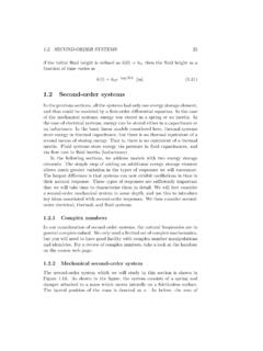
4 The roots of the denominator of vout(s) occur at s = 0 and (by use of the quadratic formula) at s1,s2= 0 0 2 1 (5) Three cases occur: > 1. The roots s1 and s2 are real. This is called the overdamped case. = 1. The roots s1 and s2 are real and repeated: s1 = s2 = 0. This case is called critically damped. < 1. The roots s1 and s2 are complex, and can be written s1,s2= 0 j 01 2 (6) This is called the underdamped case. ECEN 2830 3 Figure 2 illustrates how the positions of the roots, or poles, vary with.

5 For = , there are real poles at s = 0 and at s = . As decreases from to 1, these real poles move towards each other until, at = 1, they both occur at s = 0. Further decreasing causes the poles to become complex conjugates as given by Eq. (6). Figure 3 illustrates how the poles then move around a circle of radius 0 until, at = 0, the poles have zero real parts and lie on the imaginary axis. Figure 2 is called a root locus diagram, because it illustrates how the roots of the denominator polynomial of H(s) move in the complex plane as the parameter is varied between 0 and . Several other cases can be defined that are normally not useful in practical engineering systems.

6 When = 0, the roots have zero real parts. This is called the undamped case, and the output voltage waveform is sinusoidal. The Transient excited by the step input does not decay for large t. When < 0, the roots have positive real parts and lie in the right half of the complex plane. The output voltage Response in this case is unstable, because the expression for vout(t) contains exponentially growing terms that increase without bound for large t. Partial fraction expansion is used below to derive the output voltage waveforms for the cases that are have useful engineering applications, the overdamped, critically damped, and underdamped cases. Overdamped case, > 1 Partial fraction expansion of Eq.

7 (4) leads to Re (s)Im (s)LHPRHP 0 = = = = = j 0j 0 Fig. 2. Location of the two poles of H(s) vs. , as described by Eqs. (5) and (6). Re (s)Im (s) 0 j 0 0 0j 01 2j 0 j 01 2 Fig. 3. For 0 < 1, the complex conjugate poles lie on a circle of radius 0. ECEN 2830 4 vout(s)=K1s+K2s s1+K3s s2 (7) Here, s1 and s2 are given by Eq. (5), and the residues K1, K2 and K3 are given by K1=s1sH01+2 s 0+s 02s=0K2=s s11sH01+2 s 0+s 02s=s1K3=s s21sH01+2 s 0+s 02s=s2 (8) Evaluation of these expressions leads to K1=H0K2=s s11sH01 ss11 ss2s=s1= s2s2 s1H0K3=s s21sH01 ss11 ss2s=s2= s1s1 s2H0 (9) The inverse transform is therefore vout(t)=H0u(t)1 s2s2 s1es1t s1s1 s2es2t (10) In the overdamped case, the output voltage Response contains decaying exponential terms, and the rise time depends on the magnitudes of the roots s1 and s2.

8 The root having the smallest magnitude dominates Eq. (10): for | s1 | << | s2 |, Eq. (10) is approximately equal to vout(t) H0u(t)1 es1t (11) This is indeed what happens when >>1. Equation (11) can be expressed in terms of 0 and as vout(t) H0u(t)1 e 0t2 (12) ECEN 2830 5 When >> 1, the time constant 2 / 0 is large and the Response becomes quite slow. Critically damped case, = 1 In this case, Eq. (4) reduces to vout(s)=H0s1+s 02 (13) The partial fraction expansion of this equation is of the form vout(s)=K1s+K2s+ 02+K3s+ 0 (14) with the residues given by K1=H0K2=s+ 02H0s1+s 02s= 0= 0H0K3=ddss+ 02H0s1+s 02s= 0= H0 (15) The inverse transform is therefore vout(t)=H0u(t)1 1+ 0te 0t (16)

9 In the critically damped case, the time constant 1/ 0 is smaller than the slower time constant 2 / 0 of the overdamped case. In consequence, the Response is faster. This is the fastest Response that contains no overshoot and ringing. Underdamped case, < 1 The roots in this case are complex, as given by Eq. (6). The partial fraction expansion of Eq. (4) is of the form vout(s)=K1s+K2s+ 0 j 01 2+K2*s+ 0+j 01 2 (17) The residues are computed as follows: ECEN 2830 6 K1=H0K2=s+ 0 j 01 2H0 02ss+ 0 j 01 2s+ 0+j 01 2s= 0+j 01 2 (18) The expression for K2 can be simplified as follows: K2=H0 02 0+j 01 22j 01 2=H0 +j1 22j1 2= H021 2+j2 1 2 (19) The magnitude of K2 is K2=H021 2 (20) and the phase of K2 is K2= tan 12 1 221 2= tan 1 1 2 (21) The inverse transform is therefore vout(t)=H0u(t)1 11 2e 0tcos1 2 0t+ tan 1 1 2 (22)

10 In the underdamped case, the output voltage rises from zero to H0 faster than in the critically-damped and overdamped cases. Unfortunately, the output voltage then overshoots this value, and may ring for many cycles before settling down to the final steady-state value. ECEN 2830 7 In some applications, a moderate amount of ringing and overshoot may be acceptable. In other applications, overshoot and ringing is completely unacceptable, and may result in destruction of some elements in the System . The engineer must use his or her judgment in deciding on the best value of . 3. Step Response waveforms Equations (10), (16), and (19) were employed to plot the step Response waveforms of Fig. 4. Underdamped, critically damped, and overdamped responses are shown.