Transcription of Transmission Lines - College of Engineering and Applied ...
1 Chapter2 Transmission .. Role of Wavelength .. Modes .. Lumped Element Model .. Detail .. line Facts .. Transmission line Equations .. Propagation on a Transmission line .. to the 1D Wave Equation .. the Wave Equation (Phasor Form) .. to the Time Domain .. Lossless Microstrip line .. and Synthesis of Microstrip .. Mstrip Materials .. Tline General Case .. Reflection Coefficient .. Waves .. 2-422-1 CHAPTER 2. Transmission .. Impedance of a Lossless line .. Cases of the Lossless line .. line .. line .. of Length a Multiple of =2.. Transformer .. line :ZLDZ0.. Flow in a Lossless line .. Power .. Power .. The Smith Chart .. Parametric Equations and the -Plane .. Wave Impedance .. Impedance/Admittance Transformation .. Impedance Matching.
2 Quarter-wave Transformer Matching .. Lumped Element Matching .. Single-Stub Matching .. Transients on Transmission Lines .. Response to a Step Function .. Dr. Wickert s Archive Notes .. The Time-Domain Reflectometer .. IntroductionIn this second chapter your knowledge of circuit theory is connectedinto the study Transmission Lines having voltage and current alongthe line in terms of 1D traveling waves. The Transmission line is atwo-portcircuit used to connect a generator or transmitter signal to areceiving load over a distance. In simple terms power transfer ~A'BB' Transmission lineLoad circuitGenerator circuitReceiving-endport+ VgZgZLFigure 2-1 Atransmissionlineisatwo-portnetworkconne ctingagenerator circuit at the sending end to a load at thereceiving : Two-port model of a Transmission line . In the beginning the Transmission line is developed as a lumpedelement circuit, but then a limit is taken to convert the circuitmodel into adistributed elementcircuit Distributed element means that element values such asR,L, andCbecomeR,L, andCper unit length of the line , , /m, H/m, and F/m respectively In the lumped element model we have a pair of differentialequations to describe the voltage and current along the line Under the limiting argument which converts the circuit to dis-tributed element form, we now have a pair ofpartialdifferen-tial equations, which when solved yield a solution that is a 1 Dtraveling wave2-3 CHAPTER 2.
3 Transmission Lines Key concepts developed include: wave propagation, standingwaves, and power transfer Returning to Figure , we note that sinusoidal steady-stateis implied as the source voltage is the phasorQVg, the sourceimpedanceZgis a Th venin equivalent andZLis the loadimpedance The source may be an RF transmitter connecting to anantenna The source/load may be a pair at each end of the line whenconnecting to an Ethernet hub in wired a computer net-work The source may be power collected by an antenna and viacable to the receiver electronics, , satellite TV (DishNetwork) The Role of Wavelength When circuits are interconnected with wires (think protoboardor a printed circuit board (PCB)), is a Transmission line present? The answer isyes, for better or worse As long the circuit interconnect lengths aresmallcomparedwith the wavelength of the signals present in the circuit, lumpedelement circuit characteristics prevail Ulaby suggests Transmission line effects may be ignoredwhenl=.
4 0:01( I have been content with a =10limit) INTRODUCTION Lumped element capacitance and inductance (parasitics)due to interconnects may still alter circuit performancePower Loss and Dispersion Transmission Lines may also bedispersive, which means thepropagation velocity on the line is not constant with frequency For example the frequency components of square wave (re-call odd harmonics only) each propagate at a different velocity,meaning the waveform becomessmeared Dispersion is very important to high speed digital Transmission (fiber optic and wired networks alike) The longer the line , the greater the impactDispersionless lineShort dispersive lineLong dispersive lineFigure 2-3 Adispersionlesslinedoesnotdistortsignals passing through it regardless of its length,whereas a dispersive line distorts the shape of theinput pulses because the different frequency componentspropagate at different velocities. The degree of distortionis proportional to the length of the dispersive : The impact of Transmission line 2.
5 Transmission Propagation Modes When a time-varying signal such as sinusoid connected to (orlaunched on) a Transmission line , a propagationmodeis estab-lished Recall that both electric and magnetic fields will be present(why?) Two mode types as: (1)transvere electromagnetic (TEM)and(2) non-TEM orhigher-orderTEM Transmission LinesHigher-Order Transmission LinesMetal(g) Rectangular waveguide(h) Optical fiberConcentricdielectriclayersMetalDiel ectric spacingwhMetal2a2bDielectric spacing(a) Coaxial lineMetal strip conductorDielectric spacingwhMetal ground plane(e) Microstrip line (c) Parallel-plate line (d) Strip lineMetalDielectric spacingDielectric spacingMetal ground planeMetal(f) Coplanar waveguidedDDielectric spacing(b)Two-wire lineFigure 2-4 Afewexamplesoftransverseelectromagnetic( TEM)andhigher-order Transmission : A collection classical TEM Transmission Lines (a) (c),mircowave circuit TEM Lines (d) (f), and non-TEM Lines (g) & (h).
6 THE LUMPED ELEMENT MODEL TEM, which means electric and magnetic fields aretransverseto the direction of propagation, is the exclusive study of Chap-ter 2 VgRgRLLoadCross sectionMagnetic field linesElectric field linesGeneratorCoaxial line + Figure 2-5In a coaxial line , the electric field is in the radial directionbetweentheinnerandouterconducto rs,andthemagnetic field forms circles around the inner conductor. Thecoaxial line is a transverse electromagnetic (TEM) transmissionline because both the electric and magnetic fields are orthogonal to the direction of propagation between the generator andthe : The transverse fields of the coax. non-TEM means one or more field components lies in the di-rection of propagation, metal or optical fiber waveguides We start with alumped elementmodel of a TEM line and de-rive thetelegrapher s The Lumped Element Model TEM Transmission Lines all exhibitaxial symmetry From a circuit theory perspective the line is completely de-scribed by fourdistributed parameterquantities: R0: The effective series resistanceper unit length in /m(all conductors that make up the line cross-section are in-cluded)2-7 CHAPTER 2.
7 Transmission Lines L0: The effective series inductanceper unit length in H/m(again all conductors that make up the line cross-sectionare included) G0: The effective shunt conductanceof the line insulation(air and/or dielectric) per unit length in S/m (mhos/m?) C0: The effective shunt capacitanceper unit length be-tween the line conductors in F/m We will see that these four parameters are calculated from (1)the line cross-sectional geometry (see ) and (2) the EM con-stitutive parameters ( cand cfor conductors and , , and insulation/dielectric) For the three classical line types the four parameters are calcu-lated using the table below (also see the textJava modules1)Table :R0,L0,G0, andC0for the four classical line 2-1 Transmission - line parametersR ,L ,G ,andC for three types of UnitR Rs2 %1a+1b&2Rs d2 Rsw /mL 2 ln(b/a) ln'(D/d)+((D/d)2 1) hwH/mG 2 ln(b/a) ln*(D/d)++(D/d)2 1, whS/mC 2 ln(b/a) ln*(D/d)++(D/d)2 1, whF/mNotes: (1) Refer toFig.
8 2-4for definitions of dimensions. (2) , ,and pertain to theinsulating material between the conductors. (3)Rs=+ f c/ c.(4) cand cpertainto the conductors. (5) If(D/d)2 1, then ln-(D/d)++(D/d)2 1. ln(2D/d).1 THE LUMPED ELEMENT Coax Detail The formula forR0(see text Chapter 7) isR0 DRs2 1aC1b ( /m)whereRsis the effectivesurface resistanceof the line In text Chapter 7 it is shown thatRsDs f c c. / Note: The series resistance of the line increases as thepf Also Note: If c f cR0'0 The formula forL0(see text Chapter 5) isL0D 2 ln ba (H/m)where is the joint inductance of both conductors in the linecross-section The formula forG0(see text Chapter 4) is given byG0D2 (S/m) Note: The non-zero conductivity of the line allows current toflow between the conductors (lossless dielectric! D0andG0D0)2-9 CHAPTER 2. Transmission Lines The formula forC0(see Chapter 4), which is the shunt capaci-tance between the conductors, isC0D2 The voltage difference between the conductors sets up equaland opposite charges and it is the ratio of the charge to voltagedifference that defines the TEM line Facts Velocity of propagation relationship:L0C0D )upD1p D1pL0C0 Recall from Chapter 1cD1=p 0 0 Secondly,G0C0D Example :Coax Parameter Calculation Using Module A coaxial air line is operating at 1 MHz The inner radius isaD6mm and the outer radius isbD12mm Assume copper for the conductors ( 1) THE LUMPED ELEMENT MODEL Use the text Module to obtain the Transmission line param-eters.
9 Transmission line parameters obtained from text As an alternative, it is not much work to do the same calcula-tion in the Jupyter notebook With hand coding many options exist to do more than just ob-tainR0,L0,G0, andC0 Soon we will see other tline characteristics derived from thefour distributed element parameters2-11 CHAPTER 2. Transmission LINESF igure : Transmission line parameters from Python functioncoax_parameters() THE Transmission line The Transmission line Equations The moment you have been waiting for: solving the tline equa-tions starting from a differential length of line (classical!)R' zL' z zi(z + z, t)i(z, t)NodeN+ + G' zC' zNodeN + 1 (z, t) (z + z, t)Figure 2-8 Equivalent circuit of a two-conductortransmission line of differential length : A differential section of TEM Transmission line , zready for Kirchoff s laws. The goal of this section is to obtain the voltage across the ;t/and the current through the ;t/for any l z < 0andtvalue Note: It is customary to let the line length beland havezD0at the load end andzD lat the source end (morelater) From Kirchoff s voltage law we sum voltage drops around theloop to ;t/ R0 z ;t/ L0 @t z;t/D02-13 CHAPTER 2.
10 Transmission Lines Getting set for form a derivative in the limit, we divide by zeverywhere are rearrange z; ;t/ z @t Taking the limit as z!0gives @t From Kirchoff s current law we sum current entering minuscurrent leaving nodeNC1to ;t/ G0 z z;t/ C0 z;t/@t z;t/D0 Rearranging in similar fashion to the voltage equation, and tak-ing the limit as z!0, yields @t The above blue-boxed equations are thetelegrapher s equa-tions in the time domain A full time-domain solution is available, but will be de-ferred to later in the chapter (I like personally like startinghere) A sinusoidal steady-state solution (frequency domain) is pos-sible to if you ;t/DRe QV .z/ej!t ;t/DRe !t ; WAVE PROPAGATION ON A Transmission line withQV . the phasor components correspond-ing ; ;t/respectively The phasor form of the telegrapher s equations is simply dQV .z/dzD R0Cj!L0 G0Cj!C0 QV .z/Note:@!dsincetis suppressed in the phasor form Solving the 1D wave equation is Wave Propagation on a Transmis-sion line The phasor telegrapher equations are coupled, that is one equa-tion can be inserted into the other to eliminate eitherQV.