Transcription of Tutorial Quick Start Gephi Tutorial
1 TutorialQuick StartGephi TutorialQuick StartWelcome to this introduction Tutorial . It will guide you to the basic steps of networkvisualization and manipulation in version was used to do this Tutorial . Get Gephi Last updated March 05th, 2010* Introduction* Import file* Visualization* Layout* Ranking (color)* Metrics* Ranking (size)* Layout again* Show labels* Community-detection* Partition* Filter* Preview* Export* Save* ConclusionTutorialQuick StartOpen Graph File Download the file In the menubar, go to File Menu and Format- GEXF- GraphML- Pajek NET- GDF- GML- Tulip TLP- CSV- Compressed ZIP* Introduction* Import file* Visualization* Layout* Ranking (color)* Metrics* Ranking (size)* Layout again* Show labels* Community-detection* Partition* Filter* Preview* Export* Save* ConclusionTutorialQuick StartImport Report When your filed is opened, the report sum up data found and Number of nodes- Number of edges- Type of graph Click on OK to validate and see the graph* Introduction* Import file* Visualization* Layout* Ranking (color)* Metrics* Ranking (size)
2 * Layout again* Show labels* Community-detection* Partition* Filter* Preview* Export* Save* ConclusionTutorialQuick StartYou should now see a graphWe imported Les Miserables dataset1. Coappearance weighted network of characters in the novel Les Miserables from Victor position is random at first, so you may see a slighty different D. E. Knuth, The Stanford GraphBase: A Platform for Combinatorial Computing, Addison-Wesley, Reading, MA (1993).* Introduction* Import file* Visualization* Layout* Ranking (color)* Metrics* Ranking (size)* Layout again* Show labels* Community-detection* Partition* Filter* Preview* Export* Save* ConclusionTutorialQuick StartGraph Visualization Use your mouse to move and scale the visualization - Zoom: Mouse Wheel - Pan: Right Mouse Drag Locate the Edge Thickness slider on the bottom If you loose your graph, reset the positionZoomDrag* Introduction* Import file* Visualization* Layout* Ranking (color)* Metrics* Ranking (size)* Layout again* Show labels* Community-detection* Partition* Filter* Preview* Export* Save* Conclusion Choose Force Atlas You can see the layout properties below, leave defaultvalues.
3 Click on to launch the algorithmTutorialQuick StartLayout the graphLayout algorithms sets the graph shape, it is the most essential action. Locate the Layout module, on the left algorithmsGraphs are usually layouted with Force-based algorithms. Their principle is easy, linked nodes attract each other and non-linked nodes are pushed apart.* Introduction* Import file* Visualization* Layout* Ranking (color)* Metrics* Ranking (size)* Layout again* Show labels* Community-detection* Partition* Filter* Preview* Export* Save* ConclusionTutorialQuick StartControl the layoutThe purpose of Layout Properties is to let you control the algorithm in order to make a aesthetically pleasing representation. And now the algorithm. Set the Repulsion strengh at 10 000 to expandthe graph. Type Enter to validate the changed value.* Introduction* Import file* Visualization* Layout* Ranking (color)* Metrics* Ranking (size)* Layout again* Show labels* Community-detection* Partition* Filter* Preview* Export* Save* ConclusionTutorialQuick StartYou should now see a layouted graph* Introduction* Import file* Visualization* Layout* Ranking (color)* Metrics* Ranking (size)* Layout again* Show labels* Community-detection* Partition* Filter* Preview* Export* Save* Conclusion Locate Ranking module, in the top left.
4 Choose Degree as a rank parameter. Click on to see the StartRanking (color)Ranking module lets you configure node s color and size. You should obtain the configuration panel below:* Introduction* Import file* Visualization* Layout* Ranking (color)* Metrics* Ranking (size)* Layout again* Show labels* Community-detection* Partition* Filter* Preview* Export* Save* Conclusion Move your mouse over the gradient component. Double-click on triangles to configure the colorTutorialQuick StartLet s configure colors PaletteUse palette by right-clicking on the panel.* Introduction* Import file* Visualization* Layout* Ranking (color)* Metrics* Ranking (size)* Layout again* Show labels* Community-detection* Partition* Filter* Preview* Export* Save* Conclusion Enable table result view at the bottom toolbar Click again onTutorialQuick StartRanking result tableYou can see rank values by enabling the result table.
5 Valjean has 36 links and is the most connected node in the network.* Introduction* Import file* Visualization* Layout* Ranking (color)* Metrics* Ranking (size)* Layout again* Show labels* Community-detection* Partition* Filter* Preview* Export* Save* ConclusionWe will calculate the average path length for the network. It computes the path length for all possibles pairs of nodes and give information about how nodes are close from each other. Locate the Statistics module on the right panel. Click on near Average Path Length .TutorialQuick StartMetricsMetrics available- Diameter- Average Path Length- Clustering Coefficient- PageRank- HITS- Betweeness Centrality- Closeness Centrality- Eccentricity- Community Detection (Modularity)* Introduction* Import file* Visualization* Layout* Ranking (color)* Metrics* Ranking (size)* Layout again* Show labels* Community-detection* Partition* Filter* Preview* Export* Save* ConclusionTutorialQuick StartMetric settingsThe settings panel immediately appears.
6 Select Directed and click on OK to compute the metric.* Introduction* Import file* Visualization* Layout* Ranking (color)* Metrics* Ranking (size)* Layout again* Show labels* Community-detection* Partition* Filter* Preview* Export* Save* ConclusionTutorialQuick StartMetric resultWhen finished, the metric dis-plays its result in a report * Introduction* Import file* Visualization* Layout* Ranking (color)* Metrics* Ranking (size)* Layout again* Show labels* Community-detection* Partition* Filter* Preview* Export* Save* Conclusion Go back to Ranking Select Betweeness Centrality in the list. This metrics indicates influencial nodes for highest StartRanking (size)Metrics generates general reports but also results for each node. Thus three new values have been created by the Average Path Length algorithm we Betweeness Centrality- Closeness Centrality- Eccentricity* Introduction* Import file* Visualization* Layout* Ranking (color)* Metrics* Ranking (size)* Layout again* Show labels* Community-detection* Partition* Filter* Preview* Export* Save* ConclusionTutorialQuick StartRanking (size)The node s size will be set now.
7 Colors remain the Degree indicator. And click on to see the result. Select the diamond icon in the toolbar for size. Set a min size at 10 and a max size at 50.* Introduction* Import file* Visualization* Layout* Ranking (color)* Metrics* Ranking (size)* Layout again* Show labels* Community-detection* Partition* Filter* Preview* Export* Save* ConclusionTutorialQuick StartYou should see a colored and sized graphColor: DegreeSize: Betweeness Centrality metric* Introduction* Import file* Visualization* Layout* Ranking (color)* Metrics* Ranking (size)* Layout again* Show labels* Community-detection* Partition* Filter* Preview* Export* Save* Conclusion Go Back to the Layout panel. Check the Adjust by Sizes option and run again thealgorithm for short moment. You can see nodes are not overlapping StartLayout againThe layout is not completely satisfying, as big nodes can overlap Force Atlas algorithm has an option to take node size in account when layouting.
8 * Introduction* Import file* Visualization* Layout* Ranking (color)* Metrics* Ranking (size)* Layout again* Show labels* Community-detection* Partition* Filter* Preview* Export* Save* ConclusionLet s explore the network more in details now that colors and size indicates central nodes. Display node labels Set label size proportional to node size Set label size with the scale sliderTutorialQuick StartShow labels* Introduction* Import file* Visualization* Layout* Ranking (color)* Metrics* Ranking (size)* Layout again* Show labels* Community-detection* Partition* Filter* Preview* Export* Save* ConclusionTutorialQuick StartCommunity detectionThe ability to detect and study communities is central in network analysis. We would like to colorize clusters in our implements the Louvain method1, available from the Statistics on near the Modularity line1 Blondel V, Guillaume J, Lambiotte R, Mech E (2008) Fast unfolding of communities in large net-works.
9 J Stat Mech: Theory Exp 2008:P10008. ( ) Select Randomize on the panel. Click on OK to launch the detection.* Introduction* Import file* Visualization* Layout* Ranking (color)* Metrics* Ranking (size)* Layout again* Show labels* Community-detection* Partition* Filter* Preview* Export* Save* Conclusion Locate the Partition module on the left panel. Immediately click on the Refresh button to pop-ulate the partition StartPartitionThe community detection algorithm created a Modularity Class value for each partition module can use this new data to colorize to visualize nodes & edges columns?See columns and values for nodes and edges by looking at the Data Table Data Laboratory tab and click on Nodes to refresh the table.* Introduction* Import file* Visualization* Layout* Ranking (color)* Metrics* Ranking (size)* Layout again* Show labels* Community-detection* Partition* Filter* Preview* Export* Save* Conclusion Select Modularity Class in the partition list.
10 You can see that 9 communities were found, could be different for you. A random color has been set for each community identifier. Click on to colorize StartPartitionRight-click on the panel to access the Randomize colors action.* Introduction* Import file* Visualization* Layout* Ranking (color)* Metrics* Ranking (size)* Layout again* Show labels* Community-detection* Partition* Filter* Preview* Export* Save* ConclusionTutorialQuick StartWhat the network looks like now* Introduction* Import file* Visualization* Layout* Ranking (color)* Metrics* Ranking (size)* Layout again* Show labels* Community-detection* Partition* Filter* Preview* Export* Save* Conclusion Locate the Filters module on the right panel. Select Degree Range in the Topology category. Drag it to the Queries, drop it to Drag filter here .TutorialQuick StartFilterThe last manipulation step is filtering. You create filters that can hide nodes and egdes on the network.