Transcription of Two-Way Mixed ANOVA - Open University
1 Two-Way Mixed ANOVA analysis of variance comes in many shapes and sizes. It allows to you test whether participants perform differently in different experimental conditions. This tutorial will focus on Two-Way Mixed ANOVA . The term Two-Way gives you an indication of how many Independent Variables you have in your experimental in this case: two. The term Mixed tells you the nature of these variables. While a repeated-measures ANOVA contains only within participants variables (where participants take part in all conditions) and an independent ANOVA uses only between participants variables (where participants only take part in one condition), ' Mixed ANOVA ' contains BOTH variable types. In this case, one of each. Worked Example Previous research has found that we are better at recognising faces of our own race compared to those of other races. This tutorial will illustrate how to run a Two-Way Mixed ANOVA using this Own-Race Bias in face recognition.
2 Imagine that you wanted to investigate whether this own-race recognition advantage exists for Asian and Caucasian adults. You could show participants of both races images of faces that are both Asian and Caucasian. After a short break, you could then show them a larger pool of faces and ask participants to identify whether or not they had seen them before. In this example, there are two independent variables: Race of Participant which has two levels: Asian and Caucasian. Face Race also with two levels: Asian and Caucasian. The number of faces participants correctly recognise could be taken as the dependent variable. This is what the data collected should look like in SPSS (and can be found in the SPSS file Week 3 ORB ): As a general rule in SPSS, each row in the spreadsheet should contain all of the data provided by one participant. For within participants variables, separate columns need to represent each of the conditions of the experiment (as each participant contributes multiple data points).
3 Between participants variables are coded in a separate column, where the different levels or conditions of the IV refer to separate individuals. The different columns in SPSS display the following data: ID_No: This just refers to the ID number assigned to the participants. We use numbers as identifiers instead of participant names, as this allows us to collect data while keeping the participants anonymous. Race: This just refers to our between participants variable: participant race. As participants were either one race or the other, codes have been used to tell SPSS which condition each of the participants belonged to. In this case: 1 = Caucasian 2 = Asian Revisit the tutorial Adding Variables to see how this is done. Asian_Face: This column represents one level of our within participants IV: race of face. As participants saw all facial stimuli, conditions are represented by different columns. This column contains the number of faces participants correctly recognised when the facial stimuli were Asian.
4 Cauc_Face: This column represents one level of our within participants IV: race of face. It contains the number of faces participants correctly recognised when the facial stimuli were Caucasian. We will now walk you through how to run a Mixed ANOVA in SPSS To start the analysis , begin by CLICKING on the Analyze menu, select the General Linear Model option, and then the Repeated sub-option. You always select this option, whenever you have a within participants variable. The Repeated Measures Define Factor(s) box should now appear. This is where we tell SPSS what our within-participants IV is, and how many levels it has. It doesn t matter what name we give our variable, but it s probably a good idea to give it a sensible name, that we can interpret easily when we look at the output. In this case, let s name our variable Face_Race (the underscore is used to separate the words, as SPSS doesn't like spaces in variable names).
5 We can define our first variable by typing the name (Face_Race) into the Within-Subject Factor Name box, and entering the number of levels (2) into the Number of Levels box: CLICK on Add to add this variable to the analysis . Once you have finished defining your IV, CLICK on the Define button to continue with the analysis This opens the main ANOVA dialog box. First, we need to tell SPSS what our between-participants variable is. To do this, SELECT the Participant Race variable and move it across to the Between-Subjects Factor(s) box by CLICKING on the blue arrow to the left of the box. Next, we need to tell SPSS what the conditions of our within-participants variable are. In the Within-Subjects Variables box itself, there are a series of question marks with bracketed numbers. These numbers represent the levels of our IVs. Our task is to replace the question marks with the names of the conditions that will map onto the variable level codes.
6 To do this, SELECT the two IV conditions: Asian faces and Caucasian faces (when doing this yourself, hold down the SHIFT key to select multiple options simultaneously). Now add the conditions to the Within-Subjects Variables box by CLICKING on the top arrow button. Now we have told SPSS what is it that we want to analyse, we are almost ready to run the ANOVA . But before we do, we need to ask SPSS to produce some other information for us. First, we want to ask SPSS to produce some descriptive statistics for our different conditions ( means and standard deviations). CLICK on the Options button (highlighted in the image above) to do this. This options the Repeated Measures: Opens dialog box. To produce means for the different variables and conditions, highlight all of the factor names in the Factor(s) and Factor Interactions box, as is shown here. When doing this yourself, remember that if you hold down the Shift key you can click on and highlight all of the factors in one go.
7 (OVERALL) just gives you the overall mean of the whole data set. As we are looking for group differences, this isn't very so it isn't really worth including in this step (although you can if you like)! To move the variables across, CLICK the arrow (highlighted above). In the bottom half of the dialog box, there are a number of tick box options that you can select to get more information about the data in your output. In this example we are just going to select three. First, CLICK on Descriptive Statistics, so we can produce our means and standard deviations. Next, CLICK on Estimates of effect size to produce effect size information. Third, whenever you carry out an ANOVA which contains a between-participants variable, the assumption of homogeneity of variance must be met. This assumes that the groups you are comparing have a similar dispersion of scores. To test the assumption, CLICK on the Homogeneity Tests option now.
8 Finally, CLICK on Continue to proceed. Almost but before we can run the analysis , we need to tell SPSS to produce some more things for our output. There are a number of other buttons we could select here. If any of our IVs had more than two levels (or conditions) we would need to select the Post-Hoc tests button. But as both Race of Participant and Face Race only have two, we can skip this option on this occasion. Visit the tutorial on One-Way Independent ANOVA to see more about the Post Hoc options available in SPSS. Instead, we next want to tell SPSS to create a graph of our data for us. This will help us interpret any interaction there might be between the two Independent Variables. CLICK on the Plots button to do this. Here we are going to tell SPSS what type of graph we want. While it doesn t really matter which way round you put the variables on the graph, it is usually better to put the IV with the most levels on the horizontal axis and the other on as separate lines.
9 In this case both variables have the same number of levels: two. As such, the order really doesn t matter. As Race is already highlighted, start by moving it across to the Horizontal Axis box using the top blue arrow. Next, SELECT Face_Race and move it across to the Separate Lines box using the appropriate arrow. CLICK on the Add button to add it to the Plots box, and then CLICK Continue to proceed. We are now ready to run the analysis ! CLICK OK to continue This opens the Output window, where SPSS produces all of the statistics that you asked for: There is quite a lot of output for analysis of variance , but don t worry - this tutorial will talk you through the output you need, box by box. Within-Subjects Factors This box is just here to remind you what values you have assigned the different levels of your within-participants variable, and what they mean. You may find it useful to refer back to this when interpreting your output.
10 From looking at the box you should be able to see that for the first factor, Face_Race, there are two levels, where: 1=Asian Faces and 2=Caucasian Faces. Between-Subjects Factors This box is just here to remind you what values you have assigned the different levels of your between-participants variable, and what they mean. You may find it useful to refer back to this when interpreting your output. From looking at the box you should be able to see that for the second factor, Race, there are also two levels, where: 1 = Caucasian participants and 2 = Asian participants. Descriptive Statistics This table gives you your descriptive statistics. It s good to look at and report these, as they can give you an important insight into the pattern of your data. From this table we can see the average (mean) number of faces recognised for each of the possible variable conditions. You can also see the variation in the data ( spread of scores) for the different groups from the standard deviation.