UNSTEADY STATE HEAT CONDUCTION - NPTEL

1 MODULE 5 UNSTEADY STATE heat CONDUCTION Introduction To this point, we have considered conductive heat transfer problems in which the temperatures are independent of time. In many applications, however, the temperatures are varying with time, and we require the understanding of the complete time history of the temperature variation. For example, in metallurgy, the heat treating process can be controlled to directly affect the characteristics of the processed materials. Annealing (slow cool) can soften metals and improve ductility. On the other hand, quenching (rapid cool) can harden the strain boundary and increase strength. In order to characterize this transient behavior, the full UNSTEADY equation is needed: kqzTyTxTTa 2222221 ( ) where ck is the thermal diffusivity.

2 Without any heat generation and considering spatial variation of temperature only in x-direction, the above equation reduces to: 221xTTa ( ) For the solution of equation ( ), we need two boundary conditions in x-direction and one initial condition. Boundary conditions, as the name implies, are frequently specified along the physical boundary of an object; they can, however, also be internal a known temperature gradient at an internal line of symmetry. Biot and Fourier numbers In some transient problems, the internal temperature gradients in the body may be quite small and insignificant. Yet the temperature at a given location, or the average temperature of the object, may be changing quite rapidly with time.

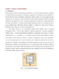
3 From eq. ( ) we can note that such could be the case for large thermal diffusivity . A more meaningful approach is to consider the general problem of transient cooling of an object, such as the hollow cylinder shown in figure TTs Fig. For very large ri, the heat transfer rate by CONDUCTION through the cylinder wall is approximately LTTlrkrrTTlrkqsioioiso)2()2( ( ) where l is the length of the cylinder and L is the material thickness. The rate of heat transfer away from the outer surface by convection is ))(2( TTlrhqso ( ) where h is the average heat transfer coefficient for convection from the entire surface. Equating ( ) and ( ) gives kLhTTTTssi = Biot number ( ) The Biot number is dimensionless, and it can be thought of as the ratio flow heat external to resistanceflow heat internal to resistanceBi Whenever the Biot number is small, the internal temperature gradients are also small and a transient problem can be treated by the lumped thermal capacity approach.

4 The lumped capacity assumption implies that the object for analysis is considered to have a single mass-averaged temperature. In the derivation shown above, the significant object dimension was the CONDUCTION path length, . In general, a characteristic length scale may be obtained by dividing the volume of the solid by its surface area: iorrL sAVL ( ) Using this method to determine the characteristic length scale, the corresponding Biot number may be evaluated for objects of any shape, for example a plate, a cylinder, or a sphere. As a thumb rule, if the Biot number turns out to be less than , lumped capacity assumption is applied. In this context, a dimensionless time, known as the Fourier number, can be obtained by multiplying the dimensional time by the thermal diffusivity and dividing by the square of the characteristic length: Fottime essdimensionl 2L ( ) Lumped thermal capacity analysis The simplest situation in an UNSTEADY heat transfer process is to use the lumped capacity assumption, wherein we neglect the temperature distribution inside the solid and only deal with the heat transfer between the solid and the ambient fluids.

5 In other words, we are assuming that the temperature inside the solid is constant and is equal to the surface temperature. The solid object shown in figure is a metal piece which is being cooled in air after hot forming. Thermal energy is leaving the object from all elements of the surface, and this is shown for simplicity by a single arrow. The first law of thermodynamics applied to this problem is dtdt timeduringobject ofenergy thermalinternal of decrease timeduringobject ofout heat Now, if Biot number is small and temperature of the object can be considered to be uniform, this equation can be written as cVdTdtTtTAhs )( ( ) or, dtcVAhTTdTs ( ) Integrating and applying the initial condition iTT )0(, tcVAhTTTtTsi )(ln ( ) Taking the exponents of both sides and rearranging, btieTTTtT )( ( ) where cVAhbs (1/s) ( ) Solid T(t) , c, V Fig.

6 T )( TTAhqs h Note: In eq. , b is a positive quantity having dimension (time)-1. The reciprocal of b is usually called time constant, which has the dimension of time. Question: What is the significance of b? Answer: According to eq. , the temperature of a body approaches the ambient temperature T exponentially. In other words, the temperature changes rapidly in the beginning, and then slowly. A larger value of b indicates that the body will approach the surrounding temperature in a shorter time. You can visualize this if you note the variables in the numerator and denominator of the expression for b. As an exercise, plot T vs. t for various values of b and note the behaviour. Rate of convection heat transfer at any given time t: TtThAtQs)()( Total amount of heat transfer between the body and the surrounding from t=0 to t: iTtTmcQ )( Maximum heat transfer (limit reached when body temperature equals that of the surrounding): iTTmcQ Numerical methods in transient heat transfer: The Finite Volume Method Consider, now, UNSTEADY STATE diffusion in the context of heat transfer, in which the temperature, T, is the scalar.

7 The corresponding partial differential equation is: SxTkxtTc ( ) The term on the left hand side of eq. ( ) is the storage term, arising out of accumulation/depletion of heat in the domain under consideration. Note that eq. ( ) is a partial differential equation as a result of an extra independent variable, time (t). The corresponding grid system is shown in fig. Fig. : Grid system of an UNSTEADY one-dimensional computational domain In order to obtain a discretized equation at the nodal point P of the control volume, integration of the governing eq. ( ) is required to be performed with respect to time as well as space. Integration over the control volume and over a time interval gives tttCVtttcvtttCVdtSdVdtdVxTkxdtdVtTc ( ) Rewritten, ttttttweewtttdtVSdtxTkAxTkAdVdttTc ( ) If the temperature at a node is assumed to prevail over the whole control volume, applying the central differencing scheme, one obtains: ttttttwWPwePEeoldPPnewdtVSdtxTTAkxTTAkVT Tc ( ) Now, an assumption is made about the variation of TP, TE and Tw with time.

8 By generalizing the approach by means of a weighting parameter f between 0 and 1: tfftdttttoldPnewPPP 1 ( ) Repeating the same operation for points E and W, xSxTTkxTTkfxTTkxTTkfxtTTcwoldWoldPweoldP oldEewnewWnewPwenewPnewEeoldPnewP )1( ( ) PP WW EE xx ww ee xx))ww xx))ee tt xx Upon re-arranging, dropping the superscript new , and casting the equation into the standard form: bTafafaTffTaTffTaTaoldPEWPoldEEEoldWWWPP )1()1()1()1(0 ( ) where PEWP aaaa 0; txcaP 0; wwWxka ; eeExka; xS b ( ) The time integration scheme would depend on the choice of the parameter f. When f = 0, the resulting scheme is explicit ; when 0 < f 1, the resulting scheme is implicit ; when f = 1, the resulting scheme is fully implicit , when f = 1/2, the resulting scheme is Crank-Nicolson (Crank and Nicolson, 1947).

9 The variation of T within the time interval t for the different schemes is shown in fig. T t+ tTP old t TP new f=0f=1 f= t Fig. : Variation of T within the time interval t for different schemes Explicit scheme Linearizing the source term as and setting f = 0 in eq. ( ), the explicit discretisation becomes: oldppuTSSb uoldPEWPoldEEoldWWPPSTaaaTaTaTa )(0 ( ) where 0 PPaa ; txcaP 0; wwWxka ; eeExka ( ) The above scheme is based on backward differencing and its Taylor series truncation error accuracy is first-order with respect to time. For stability, all coefficients must be positive in the discretized equation. Hence, 0)(0 PEWPSaaa or, 0)( eewwxkxktxc or. xktxc 2 or, kxct2)(2 ( ) The above limitation on time step suggests that the explicit scheme becomes very expensive to improve spatial accuracy.

10 Hence, this method is generally not recommended for general transient problems. Nevertheless, provided that the time step size is chosen with care, the explicit scheme described above is efficient for simple CONDUCTION calculations. Crank-Nicolson scheme Setting f = in eq. ( ), the Crank-Nicolson discretisation becomes: bTaaaTTaTTaTaPWEPoldWWWoldEEEPP 002222 ( ) where PPWEPS aaaa21)(210 ; txcaP 0; wwWxka ;eeExka ; oldppuTSSb21 ( ) The above method is implicit and simultaneous equations for all node points need to be solved at each time step. For stability, all coefficient must be positive in the discretized equation, requiring 20 WEPaaa or, kxct2)( ( ) The Crank-Nicolson scheme only slightly less restrictive than the explicit method.