Vector Error Correction Models - LearnEconometrics.com

1 Vector Error Correction Models The Vector autoregressive (VAR) model is a general framework used to describe the dynamic interrelationship among stationary variables. So, the first step in time-series analysis should be to determine whether the levels of the data are stationary. If not, take the first differences of the series and try again. Usually, if the levels (or log-levels) of your time series are not stationary, the first differences will be. If the time series are not stationary then the VAR framework needs to be modified to allow consistent estimation of the relationships among the series. The Vector Error Correction (VEC) model is just a special case of the VAR for variables that are stationary in their differences ( , I(1)). The VEC can also take into account any cointegrating relationships among the variables.

2 Consider two time-series variables, ty and .tx Generalizing the discussion about dynamic relationships to these two interrelated variables yields a system of equations: 1011112120211221yttttxttttyyxvxyxv = + + += + + + The equations describe a system in which each variable is a function of its own lag, and the lag of the other variable in the system. In this case, the system contains two variables y and x. Together the equations constitute a system known as a Vector autoregression (VAR). In this example, since the maximum lag is of order one, we have a VAR(1). If y and x are stationary, the system can be estimated using least squares applied to each equation. If y and x are not stationary in their levels, but stationary in differences ( , I(1)), then take the differences and estimate: 111121211221yttttxttttyyxvxyxv = + + = + + using least squares.

3 If y and x are I(1) and cointegrated, then the system of equations is modified to allow for the cointegrating relationship between the I(1) variables. Introducing the cointegrating relationship leads to a model known as the Vector Error Correction (VEC) model. ESTIMATING A VEC MODEL In the first example, data on the Gross Domestic Product of Australia and the are used to estimate a VEC model. We decide to use the Vector Error Correction model because (1) the time series are not stationary in their levels but are in their differences (2) the variables are cointegrated. Our initial impressions are gained from looking at plots of the two series. To get started, change the directory to the one containing your data, open a new log file, and load your data.

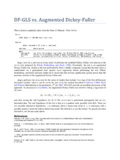
4 In this exercise we ll be using the data. use gdp, clear The data contain two quarterly time series: Australian and GDP from 1970q1 to 2004q4. As usual, create a sequence of quarterly dates: gen date = q(1970q1) + _n - 1 format %tq date tsset date Plotting the levels and differences of the two GDP series suggests that the data are nonstationary in levels, but stationary in differences. In this example, we used the tsline command with an optional scheme. A scheme holds saved graph preferences for later use. You can create your own or use one of the ones installed with Stata. At the command line you can use determine which schemes are installed on your computer by typing tsline aus usa, name(levels, replace) tsline , name(difference, replace) Neither series looks stationary in its levels.

5 They appear to have a common trend, an indication that they may be cointegrated. Unit root tests are performed using the augmented Dickey-Fuller regressions, which require some judgment about specification. The user has to decide whether to include a constant, trend or drift, and lag lengths for the differences that augment the regular Dickey-Fuller regressions. The differences are graphed and this gives some clues about specification. The graph below shows little evidence of trend or drift. 4060801001970q11980q11990q12000q1daterea l GDP of Australiareal GDP of USA Lag lengths can be chosen using model selection rules or by starting at a maximum lag length, say 4, and eliminating lags one-by-one until the t-ratio on the last lag becomes significant. dfuller aus, regress lags(1) dfuller usa, regress lags(3) Through process of elimination the decision is made to include the constant (though it looks unnecessary) and to include 1 lag for aus and 3 for the usa series.

6 In none of the ADF regressions the author estimated was either ADF statistic even close to being significant at the 5% level. Satisfied that the series are nonstationary in levels, their cointegration is explored. In each case, the null hypothesis of nonstationarity cannot be rejected at any reasonable level of significance. Next, estimate the cointegrating equation using least squares. Notice that the cointegrating relationship does not include a constant. -10121970q11980q11990q12000q1datereal GDP of Australia, Dreal GDP of USA, DMacKinnon approximate p-value for Z(t) = Z(t) Statistic Value Value Value Test 1% Critical 5% Critical 10% Critical Interpolated Dickey-Fuller Augmented Dickey-Fuller test for unit root Number of obs = 122 MacKinnon approximate p-value for Z(t) = Z(t)

7 Statistic Value Value Value Test 1% Critical 5% Critical 10% Critical Interpolated Dickey-Fuller Augmented Dickey-Fuller test for unit root Number of obs = 120. dfuller usa, regress lags(3) regress aus usa, noconst The residuals are saved in order to conduct an Engle-Granger test of cointegration and plotted. predict ehat, residual tsline ehat, name(resids, replace) The residuals have an intercept of zero and show little evidence of trend. Finally, the saved residuals are used in an auxiliary regression 1 tt teev = + The Stata command is: usa.

8 9853495 .0016566 .9820703 .9886288 aus Coef. Std. Err. t P>|t| [95% Conf. Interval] Total 124 Root MSE = Adj R-squared = Residual 123 R-squared = Model 1 Prob > F = F( 1, 123) = . Source SS df MS Number of obs = 124. reg aus usa, noconst-3-2-1012 Residuals1970q11980q11990q12000q1date regress , noconstant The t-ratio is equal to The 5% critical value for a cointegrating relationship with no intercept is and so this falls within the rejection region of the test.

9 The null hypothesis of no cointegration is rejected at the 5% level of significance. To measure the one quarter response of GDP to economic shocks we estimate the Vector Error Correction model by least squares. regress regress The VEC model results the Australian GDP are: The significant negative coefficient on 1 te indicates that Australian GDP responds to disequilibrium between the and Australia. For the : L1..0442792 ehat Coef. Std. Err. t P>|t| [95% Conf. Interval] Total 123.

10 379601302 Root MSE = .5985 Adj R-squared = Residual 122 .358201914 R-squared = Model 1 Prob > F = F( 1, 122) = Source SS df MS Number of obs = 123. reg , noconst _cons .4917059 .0579095 .3770587 .606353 L1..0475158 ehat Coef. Std. Err. t P>|t| [95% Conf. Interval] Total 122.