Transcription of Xpose 4 Bestiary - SourceForge
1 Xpose 4 BestiaryVersion Niclas Jonsson and Andrew HookerPharmacometrics Research GroupUppsala UniversityA Bestiary , or Bestiarum vocabulum, is a compendium of file ..9 Data .. 17 Overall goodness of fit .. 22runsum .. 23 Structural model .. 44 Residual model .. 71 Parameter distribution .. 81 Model .. 934 Model .. 103 Getting more help104 What is not included?105 How to makeNONMEM generate input to Xpose106 How Xpose identifiesNONMEM runs .. 106 Xpose data variables .. 106 Default variable definitions .. 106 Changing the default variable definitions .. 106 How Xpose identifies data items109 How to extend and modify the behavior of Xpose specific functions1105 IntroductionXpose is anRlibrary for post-processing ofNONMEM output. It takes one or more standardNONMEM table files as input and generates graphs or other analyses.
2 It is assumed that eachNONMEMrun can be uniquely identified by a run number (see Section How to makeNONMEM generate input to Xpose on page 106) for how to generate the appropriate input to Xpose ). Xpose is implemented using thelatticegraphics library Xpose library has five sub-libraries:xposedataContains functions for managing the input data and manipulating the Xpose generic wrapper functions around thelatticefunctions. These func-tions can be invoked by the user but require quite detailed instructions to generate thedesired functions are single purpose functions that generate specific outputgiven only the Xpose database as input. The behavior can to some extent be influencedby the , Xpose has had a text based menu interface to make it simple for theuser to invoke the Xpose specific functions. This interface is called Xpose Classic. Giventhe limitations a text based interface imposes, Xpose Classic is not very flexible but maystill be useful for quick assessment of a functions are the interface between Xpose and PsN, they do notpost-processNONMEM output but rather PsN document is intended to be a showcase for the graphical displays that can be producedusing the functions in the Xpose specific library.
3 Many of the graphs can be generated usingthe classical Xpose text based interface (albeit in a less flexible way) but not all. On the otherhand, to use the Xpose specific functions directly, it is necessary to type the functions on thecommand line and, in some cases, do some simple data management before the functions the following, each of the Xpose specific functions will be exemplified. Each display will havea legend that hopefully will be a good starting point for reports and papers. Together with eachexample will be the code used to generate the graph starting fromNONMEM table example assumes that the Xpose library has been attached:> library(xpose4)and that appropriate table files for Xpose have been produced. When preparing this docu-ment, the table files were located in the directory above from where R was running, hence thedirectory="../"argument all of the are quite a few specific functions in the Xpose library and for the sake of presentation,they have been categorized into sections:6 Data visualizationGraphs intended to plot the raw data, for example concentrations versustime or histograms of the goodness of fit assessmentXpose has a number of composite displays (multiplegraphs of different kinds on the same page) that provide diagnostics for multiple aspectsof the fit.
4 These plots go into this model diagnosticsThese are graphs that are more geared towards diagnosingthe appropriateness of the structural model diagnosticsPlots for diagnosing the statistical portions of the model (for ex-ample, residual error and between subject variability).Parameter distribution diagnosticsPlots in this section focus on the inter-individual variabil-ity comparisonGraphs for comparing various aspects of two models fit to the same developmentGraphs and functions that are supposed to help the modeler decide whatto do next with the model. Most of these functions focus on aspects of covariate note that these sections are fuzzy , in the sense that many plots could be categorizedinto several different file checkoutExploratory graphical analysis of the raw data is important and Xpose has numerous functionsto support this activity. However, most of this functionality assumes that the data is available inNONMEM table file format.
5 This is usually fine but one needs to be aware that Xpose excludesall lines withWRES=0 and only the first line for each uniqueIDnumber when plotting covariatesand/or parameters (this is the default behavior and can be changed by invoking appropriatearguments when executing the specific functions).One challenge that is related to the exploratory analysis but usually overlooked is checkingif the data file is correctly coded, for example making sure that all individuals have the doserecords they are supposed to have. Typically such checking is done by reading the data file, atedious and error prone activity. Xpose offers some support with 1:The ID-number versus the values in the AGE graph can be used to check the con-tents of the data file columns. The ID num-ber is plotted versus the values of each row inthe column. In this particular case only onepanel=column is shown but the function gen-erates one panel per column (excluding the IDcolumn) in the data the rownumber in the data file that contains the col-umn headers.
6 Check the help page for used to generate the graph:> xpdb <- (1, directory = "../")> xplot <- (obj = xpdb,+ datafile = ".. ",+ csv = F, hlin = 1, = 1)> print(xplot@plotList[[2]])9 Data visualizationSome people claim that exploratory analysis of the observed data is a sufficient data analysismethodology and that models offer only marginal additional benefit. There are of course peoplethat argue for the opposite. Regardless, exploratory graphical analysis is a powerful tool whichmay reveal a huge amount of information. It is sometimes also necessary to demonstrate thatconclusions drawn from a model based analysis is supported by the observed data itself. Onthe other hand, one may argue that the purpose of a model based analysis is to reveal thingsthat are not obvious from the raw data alone. With complicated underlying data structures anddependencies, as in PKPD data, this is even more graphical displays in this section depend only on the raw data and aim at supporting ex-ploratory graphical analysis to establish candidate models and to establish distributional repre-sentations of the underlying study vs.
7 Time (Run 1)TimeObservations05010015024681012lllll llllllllllllllllllllllllllllllllllllllll llllllllllllllllllllllllllllllllllllllll llllllllllllllllllllllllllllllllllllllll llllllllllllllllllllllllllllllllllllllll llllllllllllllllllllllllllllllllllllllll llllllllllllllllllllllllllllllllllllllll llllllllllllllllllllllllllllllllllllllll llllllllllllllllllllllllllllllllllllllll llllllllllllllllllllllllllllllllllllllll llllllllllllllllllllllllllllllllllllllll llllllllllllllllllllllllllllllllllllllll llllllllllllllllllllllllllllllllllllllll llllllllllllllllllllllllllllllllllllllll llllllllllllllllllllllllllllllllllllllll lllllllllll21435739261531646361774646177 3461214339313531726333317174650344461134 3211017461712333025044346113145361133174 7302233 Figure 2:Observed data versus time. The data points from each individual areconnected with a line and each data point is indicated by a circle.
8 Extreme datapoints (outermost 5%) are labeled with the ID-number of the corresponding indi-vidual. The red line is a graph is used for an overall visualizationof the data over the main predictor (idvoridependentvariable). To use this graph for ini-tial PK model selection it is useful to usetimeafter last doseon the x-axis. The Xpose be used to compute this. Auseful variation of this graph is to use a semi-logarithmic scale (logy=TRUE), no id-numbers(ids=FALSE) and no smooth (smooth=NULL):Code used to generate the graph:> xpdb <- (1, directory = "../")> xplot <- (xpdb, ids = TRUE)> print(xplot) predictions vs. Time (Run 1)TimePopulation predictions02040608024681012llllllllllll llllllllllllllllllllllllllllllllllllllll llllllllllllllllllllllllllllllllllllllll llllllllllllllllllllllllllllllllllllllll llllllllllllllllllllllllllllllllllllllll llllllllllllllllllllllllllllllllllllllll llllllllllllllllllllllllllllllllllllllll llllllllllllllllllllllllllllllllllllllll llllllllllllllllllllllllllllllllllllllll llllllllllllllllllllllllllllllllllllllll llllllllllllllllllllllllllllllllllllllll llllllllllllllllllllllllllllllllllllllll llllllllllllllllllllllllllllllllllllllll llllllllllllllllllllllllllllllllllllllll llllllllllllllllllllllllllllllllllllllll llllFigure 3:Population predictions versus time.
9 The predictions from each individ-ual are connected with a line and each data point is indicated by a circle. The redline is a graph is used for visualization of thepopulation predictions over the main predictor(idv). Its is more useful as method of com-municating model properties than goodness-of-fit or diagnostics since there is no referenceto which it should be compared. See also on page used to generate the graph:> xpdb <- (1, directory = "../")> xplot <- (xpdb)> print(xplot) predictions vs. Time (Run 1)TimeIndividual predictions05010015024681012llllllllllll llllllllllllllllllllllllllllllllllllllll llllllllllllllllllllllllllllllllllllllll llllllllllllllllllllllllllllllllllllllll llllllllllllllllllllllllllllllllllllllll llllllllllllllllllllllllllllllllllllllll llllllllllllllllllllllllllllllllllllllll llllllllllllllllllllllllllllllllllllllll llllllllllllllllllllllllllllllllllllllll llllllllllllllllllllllllllllllllllllllll llllllllllllllllllllllllllllllllllllllll llllllllllllllllllllllllllllllllllllllll llllllllllllllllllllllllllllllllllllllll llllllllllllllllllllllllllllllllllllllll llllllllllllllllllllllllllllllllllllllll llll214339573152061463671746461776121344 3391334423346331733461750446134132110531 7303017332233504434611314536130174733302 332 Figure 4:Individual (posterior Bayes) predictions versus time.
10 The predictionsfrom each individual are connected with a line and each data point is indicated bya circle. Extreme data points (outermost 5%) are labeled with the ID-number ofthe corresponding individual. The red line is a graph is used for visualization of theindividual predictions over the main predic-tor (idv). Its usefulness lies more in modelcommunication rather than in goodness-of-fit or diagnostics since there is no referenceto which it should be compared. See also on page used to generate the graph:> xpdb <- (1, directory = "../")> xplot <- (xpdb, ids = TRUE)> print(xplot) of covariates (Run 1)Figure 5:Histograms of WT, SEX, RACE and AGE. For the continuous covariatesthe y-axes indicates the probability density and the line is a smoothed represen-tation of this density. For the categorical covariates, the y-axes shows the countsof individuals in the respective covariate graph is used for visualization of the dis-tribution of the covariates.