Model Dy

Topic 1: The Solow Model of Economic Growth

The rst model that we will look at in this class, a model of economic growth originally developed by MIT’s Robert Solow in the 1950s, is a good example of this general approach. Solow’s purpose in developing the model was to deliberately ignore some important aspects ofmacroeconomics, suchasshort-run

  Model

Stochastic Calculus: An Introduction with Applications

model is not very far from reality then its predictions will also be close to accurate. • The model consists of mathematical assumptions about the real world. • Given these assumptions, one does mathematical analysis to see what ... dy; g(y) = Z 1 1 f(x;y)dx: The conditional density f(yjx) is de ned by f(yjx) = f(x;y) f(x):

  Model

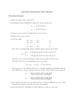
Expectation Maximization (EM) Algorithm

a model that has hidden (unobserved) variables or \arti cially" because they make the maximization more tractable. So, we may write ‘( ) ‘( b(n)) = lnf(Xj ) lnf(Xj b(n)) = ln Z f(Xjy; )f(yj )dy lnf(Xj b(n)) = ln Z f(Xjy; )f(yj ) f(yjX; b(n)) f(yjX; b(n))dy! lnf(Xj b(n)) Note that the thing in parentheses is an expectation with respect to ...

  Model, Maximization, Algorithm, Expectations, Expectation maximization

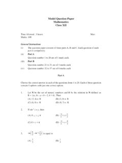
Model Question Paper Mathematics Class XII - NCERT

dy dx 26. Find ∫(sin )–1 2x dx OR Find 2 2 1 56 x dx x x + ∫ −+ 27. Evaluate 2 2 2 1-x dx ∫ − 28. Find the solution of the differential equation (x2 + y2) dx = 2xy dy OR Find the equation of the curve passing through the origin and satisfying the dif-ferential equation (1 …

  Question, Model, Paper, Mathematics, Class, Model question paper mathematics class xii

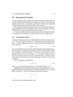
4.8 Instrumental Variables - University of California, Davis

dy=dz dx=dz: (4.46) This approach to identication of the causal parameter is given in Heckman (2000, p.58); see also the example in chapter 2.4.2. All that remains is consistent estimation of dy=dz and dx=dz. The obvi-ous way to estimate dy=dz is by OLS regression of y on z with slope estimate (z0z) 1z0y. Similarly estimate dx=dz by OLS ...

1 INTRODUCTION TO DIFFERENTIAL EQUATIONS

highest derivative y(n) in terms of the remaining n 1 variables. The differential equation, (5) where f is a real-valued continuous function, is referred to as the normal form of (4). Thus when it suits our purposes, we shall use the normal forms to represent general first- and second-order ordinary differential equations.