6 Jointly continuous random variables

Joint and Marginal Distributions - University of Arizona

Joint and Marginal Distributions October 23, 2008 We will now consider more than one random variable at a time. As we shall see, developing the theory of multivariate distributions will allow us to consider situations that model the actual collection of data and form the foundation of inference based on those data. 1 Discrete Random Variables

  Marginal

Chapter 6 Importance sampling

random variable we want to compute the mean of is of the form f(X~) where X~ is a random vector. We will assume that the joint distribution of X~ is absolutely continous and let p(~x) be the density. (Everything we will do also works for the case where the random vector X~ is discrete.) So we focus on computing Ef(X~) = Z f(~x)p(~x)dx (6.1)

  Sampling, Random

1 Sufficient statistics

conditional distribution. But then his random sample has the same distri-bution as a random sample drawn from the population (with its unknown value of θ). So statistician B can use his random sample X0 1,···,X0 n to com-pute whatever statistician A computes using his random sample X1,···,Xn, and he will (on average) do as well as ...

  Random, Conditional

A Conditional expectation

The partition theorem says that if Bn is a partition of the sample space then E[X] = X n E[XjBn]P(Bn) Now suppose that X and Y are discrete RV’s. If y is in the range of Y then Y = y is a event with nonzero probability, so we can use it as the B in the above.

Method of Moments - University of Arizona

The muon is an elementary particle with an electric charge of 1 and a spin (an intrinsic angular momentum) of 1/2. It is an unstable subatomic particle with a mean lifetime of 2.2 µs. Muons have a mass of about 200 times the mass of an electron. Since the muon’s charge and spin are the same as the electron, a muon can be

  Methods, Moment, Muon, Method of moments

Topic 15 Maximum Likelihood Estimation

Maximum Likelihood Estimation Multidimensional Estimation 1/10. Fisher Information Example Outline Fisher Information Example Distribution of Fitness E ects ... To obtain the maximum likelihood estimate for the gamma family of random variables, write the likelihood L( ; jx) = ( ) x 1 1 e x1 ( ) x 1 n e xn = ( ) n (x 1x 2 x

  Maximum, Estimation, Likelihood, Maximum likelihood estimation, Maximum likelihood

Maximum Likelihood Estimation - University of Arizona

Introduction to the Science of Statistics Maximum Likelihood Estimation 0.2 0.3 0.4 0.5 0.6 0.7 0.0e+00 5.0e-07 1.0e-06 1.5e-06 p l 0.2 0.3 0.4 0.5 0.6 0.7

  Estimation

Topic 15: Maximum Likelihood Estimation

Introduction to Statistical Methodology Maximum Likelihood Estimation Exercise 3. Check that this is a maximum. Thus, p^(x) = x: In this case the maximum likelihood estimator is also unbiased. Example 4 (Normal data). Maximum likelihood estimation can be applied to a vector valued parameter. For a simple

  Topics, Maximum, Estimation, Likelihood, Maximum likelihood estimation, Topic 15

Innovative Methods of Teaching - University of Arizona

The reason being that martyr is engaged in defense work while an alim (scholar) builds individuals and nations along positive lines. In this way he bestows a real life to the world. “Education is the manifestation of perfection already in man” – (Swami Vivekananda)

  Martyr

Probability Theory - University of Arizona

Probability Theory December 12, 2006 Contents 1 Probability Measures, Random Variables, and Expectation 3 ... Definition 1.18. Let f : (S,S) → (T,T ) be a function between measure spaces, then f is called measurable if f−1(B) ∈ S for every B ∈ T . (1.6) If (S,S) has a probability measure, then f is called a random variable.

  Measure, Theory, Space, Measurable, Measure spaces

Chapter 5: JOINT PROBABILITY DISTRIBUTIONS Part 1 ...

Mean from a Joint Distribution If Xand Y are continuous random variables with joint probability density function fXY(x;y), then E(X) = Z 1 1 xfX(x) dx = Z 1 1 Z 1 1 xfXY(x;y) dydx HINT: E(X) and V(X) can be obtained by rst calculating the marginal probability distribution of X, or fX(x). 22

  Distribution, Joint, Continuous, Joint distributions

Univariate Distribution Relationships

verse cumulative distribution function of a continuous ran-dom variable can be expressed in closed form. For a dis-crete random variable, this property indicates that a variate can be generated in an O(1)algorithm that does not cycle through the support values or …

  Distribution, Continuous

21 The Exponential Distribution

distribution if it has probability density function f X(x|λ) = ˆ λe−λx for x>0 0 for x≤ 0, where λ>0 is called the rate of the distribution. In the study of continuous-time stochastic processes, the exponential distribution is usually used to model the time until something hap-pens in the process. The mean of the Exponential(λ ...

  Distribution, Continuous, Exponential, Exponential distribution

Discrete and Continuous Random Variables

the probability distribution function, f(x), for continuous R.V. X. The total area under f(x) is 1.0 a b c . 15.063 Summer 2003 1818 The Uniform Distribution a) What is the mean transit time? X is uniform on [a,b] if X is equally likely to take any value in the range from a to b.

  Distribution, Continuous

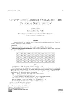
Continuous Random Variables: The Uniform Distribution

De nition 2: Uniform Distribution A continuous random ariablev V)(R that has equally likely outcomes over the domain, a<x<b. Often referred as the Rectangular distribution because the graph of the pdf has the form of a rectangle. Notation: X~U (a;b). The mean is = a+b 2 and the standard deviation is ˙= q (ba) 2 12 The probability density ...

  Distribution, Uniform, Variable, Continuous, Random, Continuous random variables, The uniform distribution

Probability Distributions: Discrete vs. Continuous

A continuous probability distribution differs from a discrete probability distribution in several ways. The probability that a continuous random variable will assume a particular value is zero. As a result, a continuous probability distribution cannot be expressed in tabular form.

  Distribution, Continuous

Lecture 4: Random Variables and Distributions

The expected or mean value of a continuous rv X with pdf f(x) is: Discrete ... probability distribution - referred to as a sampling distribution •Let’s focus on the sampling distribution of the mean,! X . Behold The Power of the CLT •Let X 1,X 2

  Distribution, Continuous

Chapter 3 Continuous Random Variables

Random variable Xis continuous if probability density function (pdf) fis continuous at all but a nite number of points and possesses the following properties: f(x) 0, for all x, R 1 1 f(x) dx= 1, P(a<X b) = R b a f(x) dx The (cumulative) distribution function (cdf) for random variable Xis F(x) = P(X x) = Z x 1 f(t) dt; and has properties lim x ...

  Distribution, Continuous

Lecture 4: Poisson Approximation to Binomial Distribution ...

Binomial Distribution • For Binomial Distribution with large n, calculating the mass function is pretty nasty • So for those nasty “large” Binomials (n ≥100) and for small π (usually ≤0.01), we can use a Poisson with λ = nπ (≤20) to approximate it!

  Distribution