6 Jointly continuous random variables

Joint and Marginal Distributions - University of Arizona

Joint and Marginal Distributions October 23, 2008 We will now consider more than one random variable at a time. As we shall see, developing the theory of multivariate distributions will allow us to consider situations that model the actual collection of data and form the foundation of inference based on those data. 1 Discrete Random Variables

  Marginal

Chapter 6 Importance sampling

random variable we want to compute the mean of is of the form f(X~) where X~ is a random vector. We will assume that the joint distribution of X~ is absolutely continous and let p(~x) be the density. (Everything we will do also works for the case where the random vector X~ is discrete.) So we focus on computing Ef(X~) = Z f(~x)p(~x)dx (6.1)

  Sampling, Random

1 Sufficient statistics

conditional distribution. But then his random sample has the same distri-bution as a random sample drawn from the population (with its unknown value of θ). So statistician B can use his random sample X0 1,···,X0 n to com-pute whatever statistician A computes using his random sample X1,···,Xn, and he will (on average) do as well as ...

  Random, Conditional

A Conditional expectation

The partition theorem says that if Bn is a partition of the sample space then E[X] = X n E[XjBn]P(Bn) Now suppose that X and Y are discrete RV’s. If y is in the range of Y then Y = y is a event with nonzero probability, so we can use it as the B in the above.

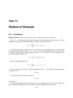
Method of Moments - University of Arizona

The muon is an elementary particle with an electric charge of 1 and a spin (an intrinsic angular momentum) of 1/2. It is an unstable subatomic particle with a mean lifetime of 2.2 µs. Muons have a mass of about 200 times the mass of an electron. Since the muon’s charge and spin are the same as the electron, a muon can be

  Methods, Moment, Muon, Method of moments

Topic 15 Maximum Likelihood Estimation

Maximum Likelihood Estimation Multidimensional Estimation 1/10. Fisher Information Example Outline Fisher Information Example Distribution of Fitness E ects ... To obtain the maximum likelihood estimate for the gamma family of random variables, write the likelihood L( ; jx) = ( ) x 1 1 e x1 ( ) x 1 n e xn = ( ) n (x 1x 2 x

  Maximum, Estimation, Likelihood, Maximum likelihood estimation, Maximum likelihood

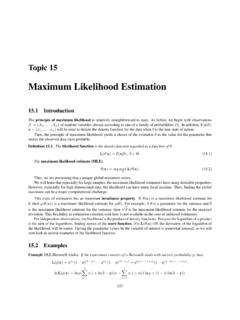
Maximum Likelihood Estimation - University of Arizona

Introduction to the Science of Statistics Maximum Likelihood Estimation 0.2 0.3 0.4 0.5 0.6 0.7 0.0e+00 5.0e-07 1.0e-06 1.5e-06 p l 0.2 0.3 0.4 0.5 0.6 0.7

  Estimation

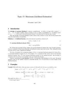
Topic 15: Maximum Likelihood Estimation

Introduction to Statistical Methodology Maximum Likelihood Estimation Exercise 3. Check that this is a maximum. Thus, p^(x) = x: In this case the maximum likelihood estimator is also unbiased. Example 4 (Normal data). Maximum likelihood estimation can be applied to a vector valued parameter. For a simple

  Topics, Maximum, Estimation, Likelihood, Maximum likelihood estimation, Topic 15

Innovative Methods of Teaching - University of Arizona

The reason being that martyr is engaged in defense work while an alim (scholar) builds individuals and nations along positive lines. In this way he bestows a real life to the world. “Education is the manifestation of perfection already in man” – (Swami Vivekananda)

  Martyr

Probability Theory - University of Arizona

Probability Theory December 12, 2006 Contents 1 Probability Measures, Random Variables, and Expectation 3 ... Definition 1.18. Let f : (S,S) → (T,T ) be a function between measure spaces, then f is called measurable if f−1(B) ∈ S for every B ∈ T . (1.6) If (S,S) has a probability measure, then f is called a random variable.

  Measure, Theory, Space, Measurable, Measure spaces

18.440: Lecture 18 Uniform random variables

Uniform random variables and percentiles. Toss n = 300 million Americans into a hat and pull one out. uniformly at random. Is the height of the person you choose a uniform random variable? Maybe in an approximate sense? No. Is the percentile of the person I choose uniformly random? In. other words, let p be the fraction of people left in the hat

  Uniform, Variable, Random, Uniform random variables, Uniform random

Discrete and Continuous Random Variables

15.063 Summer 2003 1616 Continuous Random Variables A continuous random variable can take any value in some interval Example: X = time a customer spends waiting in line at the store • “Infinite” number of possible values for the random variable.

  Variable, Continuous, Random, Random variables, Continuous random variables

S1 Discrete random variables - PMT

S1 Discrete random variables . PhysicsAndMathsTutor.com (e) Var(X) (3) (Total 10 marks) 14. A fairground game involves trying to hit a moving target with a gunshot.

  Variable, Random, Random variables

PROBABILITY AND STATISTICS FOR ECONOMISTS

Preface This textbook is the first in a two-part series covering the core material typically taught in a one-year Ph.D. course in econometrics.

Chapter 2 The Maximum Likelihood Estimator

Example 2.2.1 (The uniform distribution) Consider the uniform distribution, which has the density f(x; )= 1I [0, ](x). Given the iid uniform random variables {X i} the likelihood (it is easier to study the likelihood rather than the log-likelihood) is L n(X n; )= 1 n Yn i=1 I [0, ](X i). Using L n(X n

  Uniform, Maximum, Variable, Estimator, Random, Likelihood, Maximum likelihood estimator, Uniform random variables

Chapter 3 Continuous Random Variables

76 Chapter 3. Continuous Random Variables (LECTURE NOTES 5) with associated standard deviation, ˙= p ˙2. The moment-generating function is M(t) = E 1 etX = Z 1 etXf(x) dx for values of tfor which this integral exists. Expected value, assuming it exists, of a function uof Xis E[u(X)] = Z 1 1 u(x)f(x) dx The (100p)th percentile is a value of ...

  Variable, Random, Random variables

Properties of Expected values and Variance

Another way to look at binomial random variables; Let X i be 1 if the ith trial is a success and 0 if a failure. Note that E(X i) = 0 q + 1 p = p. Our binomial variable (the number of successes) is X = X 1 + X 2 + X 3 + :::+ X n so E(X) = E(X 1) + E(X 2) + E(X 3) + :::+ E(X n) = np: What about products? Only works out well if the random ...

  Variable, Random, Random variables

Lecture 15: Order Statistics - Duke University

n iid random variables X k is the kth smallest X, usually called the kth order statistic. X (1) is therefore the smallest X and X (1) = min(X 1;:::;X n) Similarly, X (n) is the largest X and X (n) = max(X 1;:::;X n) Statistics 104 (Colin Rundel) Lecture 15 March 14, 2012 2 / 24 Section 4.6 Order Statistics Notation Detour For a continuous ...

  Variable, Random, Random variables