
Chapter 2 Ordinary Differential Equations
governing equations with one independent variable are called ordinary differential equations. Because of this, we will study the methods of solution of differential equations. Differential equation Definition 1 A differential equation is an equation, which includes at least one derivative of an unknown function. Example 1: a) ( ) x xy x e dx
Download Chapter 2 Ordinary Differential Equations

Information
Domain:
Source:
Link to this page:
Documents from same domain

table of laplace transforms - Educating Global Leaders
www.et.byu.edutable of laplace transforms 1 f(t) f(s) tn n = 1,2,... s > 0 † n! † sn+1 1 s2 † t † ta † a>-1 † G(a+1) sa+1 s > 0 † eat † teat † tneat † 1 s-a † 1 (s-a)2 † n! ... Laplace transform is calculated with the command laplace (f(t),t,s): f(t) denotes the function to be transformed,

Chapter 5 Special Functions
www.et.byu.eduChapter 5 SPECIAL FUNCTIONS Chapter 5 SPECIAL FUNCTIONS Introduction In this chapter we summarize information about several functions which are widely used for mathematical modeling in engineering. Some of them play a supplemental role, while the others, such as the Bessel and Legendre functions, are of primary importance. ...

CHAPTER 3 PRESSURE AND FLUID STATICS
www.et.byu.edu(a) The fluid level in the arm attached to the tank is higher (vacuum): PP P . . .abs atm vac 12 7 1 26 11 44 psia 11.4 psia (b) The fluid level in the arm attached to the tank is lower: PP P . . .abs gage atm 12 7 1 26 13 96 psia 14.0 psia Discussion The final results are reported to three significant digits. Note

Second Order Systems
www.et.byu.eduSecond Order Systems Second Order Equations 2 2 +2 +1 = s s K G s τ ζτ Standard Form τ2 d 2 y dt2 +2ζτ dy dt +y =Kf(t) Corresponding Differential Equation K = Gain τ= Natural Period of Oscillation ζ= Damping Factor (zeta) Note: this has to be 1.0!!!
CHAPTER 6 MOMENTUM ANALYSIS OF FLOW SYSTEMS
www.et.byu.edutorque, the angular momentum remains constant, but the angular velocity changes in accordance with I = constant where I is the moment of inertia of the body. Discussion Angular momentum is analogous to linear momentum in this way: Linear momentum does not change unless a force acts on it. Angular momentum does not change unless a torque acts on it.

CHAPTER 5 BERNOULLI AND ENERGY EQUATIONS
www.et.byu.edu5-1 Solutions Manual for Fluid Mechanics: Fundamentals and Applications Third Edition Yunus A. Çengel & John M. Cimbala McGraw-Hill, 2013 CHAPTER 5 BERNOULLI AND ENERGY EQUATIONS PROPRIETARY AND CONFIDENTIAL This Manual is the proprietary property of The McGraw-Hill Companies, Inc.

1 HOMOGENEOUS TRANSFORMATIONS - Ira A. Fulton …
www.et.byu.edusimple 4 x 4 transformation is used in the geometry engines of CAD systems and in the kinematics model in robot controllers. It is very useful for examining rigid-body position and orientation (pose) of a sequence of robotic links and joint frames. Script Notation: Pre super- and pre sub-scripts are often used to denote frames of reference B
Related documents
ELEMENTARY DIFFERENTIAL EQUATIONS
ramanujan.math.trinity.edumethods that can be applied in later courses. Only a relatively small part of the book is devoted to the derivation of specific differential equations from mathematical models, or relating the differential equations that we study tospecific applications. In this section we mention a few such applications.
NUMERICALSOLUTIONOF ORDINARYDIFFERENTIAL …
homepage.divms.uiowa.edutext, we consider numerical methods for solving ordinary differential equations, that is, those differential equations that have only one independent variable. The differential equations we consider in most of the book are of the form Y′(t) = f(t,Y(t)), where Y(t) is an unknown function that is being sought. The given function f(t,y)
Writing Chapter 3 Chapter 3: Methodology
education.nova.eduOrdinary details of each teacher’s work experience were included, and standard categories for cultural descriptions were used. The final interpretive report was then reviewed, which allowed the researcher to provide subjective explanations of the data representing the nature of teacher retention.
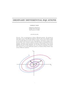
ORDINARY DIFFERENTIAL EQUATIONS
users.math.msu.eduSummary. This is an introduction to ordinary di erential equations. We describe the main ideas to solve certain di erential equations, like rst order scalar equations, second order linear equations, and systems of linear equations. We use power series methods to solve variable coe cients second order linear equations. We introduce Laplace trans-
LECTURE NOTES ON MATHEMATICAL METHODS
www3.nd.edusurvey topics in applied mathematics, including multidimensional calculus, ordinary differ-ential equations, perturbation methods, vectors and tensors, linear analysis, linear algebra, and non-linear dynamic systems. In short, the course fully explores linear systems and con-
Runge–Kutta methods for ordinary differential equations
www.math.auckland.ac.nzMethods have been found based on Gaussian quadrature. Later this extended to methods related to Radau and Lobatto quadrature. A-stable methods exist in these classes. Because of the high cost of these methods, attention moved to diagonally and singly implicit methods. Runge–Kutta methods for ordinary differential equations – p. 5/48

Programming Numerical Methods in MATLAB - Amazon S3
s3-us-west-1.amazonaws.comJan 05, 2018 · Numerical methods have great and increasing importance in the scientific and engineering computations. This is because most of the mathematical formulas developed from the real ... Higher-Order Ordinary Differential Equations 61 . For the full version of the e-book,

M.I.T. 18.03 Ordinary Di erential Equations
math.mit.educally. The numerical methods then give the actual graphs to as great an accuracy as desired; the computer does the numerical work, and plots the solutions. 1. Graphical methods. The graphical methods are based on the construction of what is called a direction field for the equation (1).

Numerical Solution of Ordinary Differential Equations
people.maths.ox.ac.ukApproximation of initial value problems for ordinary differential equations: one-step methods including the explicit and implicit Euler methods, the trapezium rule method, and Runge–Kutta methods. Linear multi-step methods: consistency, zero-stability and convergence; absolute stability. Predictor-corrector methods.
Textbook notes for Runge-Kutta 2nd Order Method for ...
mathforcollege.comOct 13, 2010 · The Runge-Kutta 2nd order method is a numerical technique used to solve an ordinary differential equation of the form . f (x, y), y(0) y 0 dx dy = = Only first order ordinary differential equations can be solved by uthe Runge-Kutta 2nd sing order method. In other sections, we will discuss how the Euler and Runge-Kutta methods are