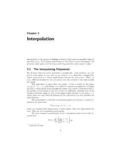
Chapter 3 Interpolation - MathWorks
2 Chapter 3. Interpolation There are n terms in the sum and n − 1 terms in each product, so this expression defines a polynomial of degree at most n−1.If P(x) is evaluated at x = xk, all the products except the kth are zero.Furthermore, the kth product is equal to one, so the sum is equal to yk and the interpolation conditions are satisfied. For example, consider the following data set.
Download Chapter 3 Interpolation - MathWorks

Information
Domain:
Source:
Link to this page:
Documents from same domain
Modeling a 4G LTE System in MATLAB - MathWorks
www.mathworks.com4 Motivation – Very high capacity & throughput – Support for video streaming, web browsing, VoIP, mobile apps A true global standard – Contributions from all across globe

Generating LTE Waveforms - MathWorks
www.mathworks.comWhen we select an RMC, all the parameters are set up as defined in 3GPP TS 36.101 [1] Annex A.3. For R.13, the number of resource blocks is set to 50, the number of antennas to 4, and so forth.
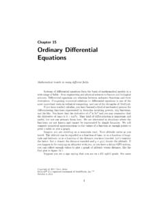
Chapter 15 Ordinary Differential Equations - mathworks.com
www.mathworks.coma second order method with a third order method to estimate the step size, while ode45 compares a fourth order method with a fifth order method. The letter “s” in the name of some of the ode functions indicates a stiff solver.

Using Model-Based Calibration Toolbox Multimodels for ...
www.mathworks.comUsing Model-Based Calibration Toolbox Multimodels for Cycle-Optimized Diesel Calibration Joshua P. Styron Ford Motor Company ABSTRACT Modern diesel engines have many degrees of freedom that must be simultaneously adjusted to optimize efficiency,

Control System Design and Rapid Prototyping Using Simulink
www.mathworks.com11 System Identification Integrated into PID Tuner in Simulink Control Design Compute plant transfer function from simulation input-output data when exact
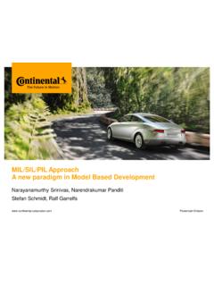
MIL/SIL/PIL Approach A new paradigm in Model Based …
www.mathworks.comBitte decken Sie die schraffierte Fläche mit einem Bild ab. Please cover the shaded area with a picture. (24,4 x 11,0 cm) MIL/SIL/PIL Approach A new paradigm in Model Based Development

Developing Battery Management Systems with Simulink and ...
www.mathworks.comWHITE PAPER | 5 Figure 2. Equivalent circuit of a battery with three distinct time constants, internal resistance, and open circuit potential. By incorporating Simscape Electrical™ components, you can scale up from the unit cell level to the module and pack level and intuitively combine cells with surrounding circuitry.
Chapter 12 Game of Life - MathWorks
www.mathworks.comalternations of a society of living organisms, it belongs to a growing class of what are called “simulation games” – games that resemble real-life processes. To play life you must have a fairly large checkerboard and a plentiful supply of flat counters of two colors. Of course, today we can run the simulations on our computers.

R2020b Updates Release Notes - MathWorks
www.mathworks.comTo learn more about Updates, see Updates: Frequently Asked Questions. Important Limitations • MATLAB Parallel Server, MATLAB Parallel Server for Amazon EC2, and MATLAB Parallel Server - Private Cloud: Install the Update on all client and worker installations.
MATLAB Basic Functions Reference - MathWorks
www.mathworks.comaxis(lim), axis style Set axis limits and style text(x,y,"txt") Add text grid on/off Show axis grid hold on/off Retain the current plot when adding new plots subplot(m,n,p), tiledlayout(m,n) Create axes in tiled positions yyaxis left/right Create second y-axis figure Create figure window gcf, gca Get current figure, get current axis clf Clear ...
Related documents

Graphing Polynomial Functions
static.bigideasmath.comSection 4.1 Graphing Polynomial Functions 161 Solving a Real-Life Problem The estimated number V (in thousands) of electric vehicles in use in the United States can be modeled by the polynomial function V(t) = 0.151280t3 − 3.28234t2 + 23.7565t − 2.041 where t represents the year, with t = 1 corresponding to 2001. a. Use a graphing calculator to graph the function for …
Unit 3 Chapter 6 Polynomials and Polynomial Functions
www.scasd.orgCP A2 Unit 3 Ch 6 Worksheets and Warm Ups 1 Unit 3 – Chapter 6 Polynomials and Polynomial Functions Worksheet Packet Mrs. Linda Gattis LHG11@scasd.org Learning Targets: Polynomials: The Basics 1. I can classify polynomials by degree and number of terms. 2. I can use polynomial functions to model real life situations and make predictions 3.
Chapter 3 Interpolation - MIT OpenCourseWare
ocw.mit.eduIn this chapter, we will immediately put interpolation to use to formulate high-order quadrature and di erentiation rules. 3.1 Polynomial interpolation Given N+ 1 points x j 2R, 0 j N, and sample values y j = f(x j) of a function at these points, the polynomial interpolation problem consists in nding a polynomial p

Chapter 3
www.math.ucdavis.edu22 3. Continuous Functions If c ∈ A is an accumulation point of A, then continuity of f at c is equivalent to the condition that lim x!c f(x) = f(c), meaning that the limit of f as x → c exists and is equal to the value of f at c. Example 3.3. If f: (a,b) → R is defined on an open interval, then f is continuous on (a,b) if and only iflim x!c f(x) = f(c) for every a < c < b ...
MATLAB Commands and Functions - Omicron Chapter
www.hkn.umn.eduPolynomial and Regression Functions / 14 Interpolation Functions / 14 Numerical Integration Functions / 14 Numerical Differentiation Functions / 14 ODE Solvers / 15 Predefined Input Functions / 15 Symbolic Math Toolbox Functions for Creating and Evaluating Symbolic Expressions / 16

Chapter 3 Polynomial Functions - MS Guides
wp.srsd119.caChapter 3 Polynomial Functions Section 3.1 Characteristics of Polynomial Functions Section 3.1 Page 114 Question 1 A polynomial function has the form f(x) = anx n + a n – 1x n – 1 + a n – 2x n – 2 + … + a 2x 2 + a 1x + a0, where an is the leading coefficient; a0 is the constant; and the degree of the polynomial, n,

Chapter 5 Techniques of Differentiation
www.math.smith.eduWe also saw in chapter 3 that the polynomial 5x3−7x2+3 can be thought of as an algebraic combination of simple functions. We can build an even...and algebraically more complicated function by forming a quotient with this polynomial in the numerator and the difference of the functions sinx and ex in the denominator. The result is 5x3 − 7x2 ...

Chapter 3 - Interpolation
www.cs.usask.ca3.1 The Interpolating Polynomial Interpolationis the process of de ning a function that \connects the dots" between speci ed (data) points. In this chapter, we focus on two closely related interpolants, thecubic splineand theshape-preserving cubic splinecalled \pchip". Two distinct points uniquely determine a straight line.

Unit 3 (Ch 6) Polynomials and Polynomial Functions
www.scasd.orgCP A2 Unit 3 (chapter 6) Notes 11 LT2. I can use polynomial functions to model real life situations and make predictions Comparing Models Use a graphing calculator to find the best regression equation for the following data. Compare linear, quadratic and cubic regressions.