
Chapter 4: Unconstrained Optimization - McMaster University
5 Steepest Ascent (Descent) Method Idea: starting from an initial point, find the function maximum (minimum) along the steepest direction so that shortest searching time is required. Steepest direction: directional derivative is maximum in that direction — gradi-ent direction. f() = ¢µ + @f @y ¢ =[] ¢]
Download Chapter 4: Unconstrained Optimization - McMaster University

Information
Domain:
Source:
Link to this page:
Documents from same domain

Functional Magnetic Resonance Imaging - …
www.ece.mcmaster.ca• Functional magnetic resonance imaging, or fMRI, is a technique for measuring brain activity. • It works by detecting the changes in blood oxygenation and flow

LECTURE 12: Reflector Antennas - McMaster …
www.ece.mcmaster.caNikolova 2016 4 The simplest reflector antenna consists of two components: a reflecting surface and a much smaller feed antennaat the reflector’s focal point.

Magnetism and Electromagnetism - McMaster University
www.ece.mcmaster.caMagnetism and Electromagnetism Unit 1 – Magnetism 2 Two of the most familiar types of magnets are the bar magnet (A) and the horseshoe magnet (B). Their names reflect their physical shape. A magnet's pole is the area where its magnetic force is strongest. Magnets of virtually any shape
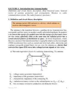
Introduction into the Antenna Studies - McMaster University
www.ece.mcmaster.caLECTURE 1: Introduction into Antenna Studies (Definition and circuit theory description. Brief historical notes. General ... Nikolova 2018 12 . ... E. Reflector antennas A reflector is used to concentrate the EM energy in a focal point where the receiver or the feed is located. Optical astronomers have long known that a

Control System Design - McMaster University
www.ece.mcmaster.caChapter 2 Goodwin, Graebe, Salgado©, Prentice Hall 2000 Modeling To make progress on the control system design problem, it is first necessary to gain an understanding of how the process operates.

Control System Design - McMaster University
www.ece.mcmaster.caControl System Design Notes for Lecture #31 Monday, March 29, 2004 Dr. Ian C. Bruce ... Digital Control Design by Pole Assignment ... There are a number of ways of designing digital control systems: design in continuous time and discretize the controller prior to

Chapter 6: Curve Fitting - McMaster University
www.ece.mcmaster.ca† Interpolation Given data for discrete values, fit a curve or a series of curves that pass di- ... † The problem of determining a least-squares second order polynomial is equiv-alent to solving a system of 3 simultaneous linear equations.

Chapter 5: Numerical Integration and Differentiation
www.ece.mcmaster.caChapter 5: Numerical Integration and Differentiation PART I: Numerical Integration Newton-Cotes Integration Formulas The idea of Newton-Cotes formulas is to replace a complicated function or tabu-lated data with an approximating function that is easy to integrate. I = Z b a f(x)dx … Z b a fn(x)dx where fn(x) = a0 +a1x+a2x2 +:::+anxn. 1 The ...
Related documents

METHODS FOR NON-LINEAR LEAST SQUARES PROBLEMS - …
www2.imm.dtu.dkThe Steepest Descent method From (2.5) we see that when we perform a step fi hwith positive fi, then the relative gain in function value satisfies lim fi!0 F(x) ¡F(x+fih) fikhk = ¡ 1 khk h>F0(x)=¡kF0(x)kcosµ; where µis the angle between the vectors h and F0(x). This shows that we get the greatest gain rate if µ=…, ie if we use the ...

Experiment 1: Equipotential Lines and Electric Fields
ocw.mit.edusteepest runs? Which have the most level sections? How do you know? (b) How steep is the steepest street at its steepest (what is its slope in ft/mi)? (c) Which would take more work (in the physics sense): walking 3 blocks south from Laguna and Jackson or 1 block west from Clay and Franklin? 2. Equipotentials, Electric Fields and Charge
The Steepest Descent Algorithm for Unconstrained ...
ocw.mit.eduUsing the steepest descent algorithm to minimize f (x) starting from x1 =(x1 1 1,x2)=(0, 10), and using a tolerance of =10−6, we compute the iterates shown in Table 2 and in Figure 2: For a convex quadratic function f (x)= 1xT Qx−cT x, the contours of the 2 function values will be shaped like ellipsoids, and the gradient vector ∇f (x)
A Brief Description of the Levenberg-Marquardt Algorithm ...
users.ics.forth.grthe algorithm behaves like a steepest descent method: slow, but guaranteed to 1. converge. When the current solution is close to the correct solution, it becomes a Gauss-Newton method. Next, a short description of the LM algorithm based on the material in [5] is supplied. Note, however, that a detailed analysis of the LM
Logistic regression - University of California, San Diego
vulstats.ucsd.edulogistic regression curve is steepest at this halfway point. The function logit−1(x)= ex 1+ex transforms continuous values to the range (0,1), which is necessary, since probabilities must be between 0 and 1. This is illustrated for the election example in Figure 5.1 and more theoretically in Figure 5.2. Equivalently, model (5.1) can be ...

Table 1.3 Primary Energy Consumption by Source ...
www.eia.govU. S. Energy Information Administration / Monthly Energy Review January 2022 7 Table 1.3 Primary Energy Consumption by Source (Quadrillion Btu)
Levenberg–Marquardt Training
www.eng.auburn.eduWith the definition of gradient g in (12.3), the update rule of the steepest descent algorithm could be written as w w k k+1 = −αg k (12.4) where α is the learning constant (step size). The training process of the steepest descent algorithm is asymptotic convergence. Around the solu-