-dimensional Fourier Transform
n-dimensional Fourier Transform 8.1 Space, the Final Frontier To quote Ron Bracewell from p. 119 of his book Two-Dimensional Imaging, “In two dimensions phenomena are richer than in one dimension.” True enough, working in two dimensions offers many new and rich possibilities.
Download -dimensional Fourier Transform

Information
Domain:
Source:
Link to this page:
Documents from same domain
Probability Theory Review for Machine Learning
see.stanford.eduProbability Theory Review for Machine Learning Samuel Ieong November 6, 2006 1 Basic Concepts Broadly speaking, probability theory is the mathematical study of uncertainty.

Lecture 3 Linear Equations and Matrices
see.stanford.eduso multiplication by matrix inverse solves a set of linear equations some comments: • x = A−1b makes solving set of 100 linear equations in 100 variables look simple, but the notation is hiding alot of work!

Much of this handout was written by Justin Manus and ...
see.stanford.eduDownloading Eclipse Much of this handout was written by Justin Manus and Brandon Burr. This quarter we’ll be using Stanford’s customized version of Eclipse to build our programs. Eclipse is an enormously popular industrial strength Java environment with many, many features. Fortunately, Eclipse is also open source—anyone is free to change

cvx Users’ Guide - Stanford Engineering Everywhere
see.stanford.edu1.2 What is disciplined convex programming? Disciplined convex programming is a methodology for constructing convex optimiza-tion problems proposed by Michael Grant, Stephen Boyd, and …
EE364a Homework 3 solutions
see.stanford.eduEE364a Homework 3 solutions 3.42 Approximation width. Let f0,...,fn: R → R be given continuous functions. We ... Use part (c) to verify that f ... 4.8 Some simple LPs. Give an explicit solution of each of the following LPs. (a) Minimizing a linear function over an affine set. minimize cTx subject to Ax = b.

CS229 Lecture notes - Stanford Engineering Everywhere
see.stanford.eduwe decide to approximate y as a linear function of x: hθ(x) = θ0 +θ1x1 +θ2x2 Here, the θi’s are the parameters (also called weights) parameterizing the space of linear functions mapping from X to Y. When there is no risk of confusion, we will drop the θ …

CS 229, Public Course Problem Set #1 Solutions: Supervised ...
see.stanford.edu2. Locally-weighted logistic regression In this problem you will implement a locally-weighted version of logistic regression, where we weight different training examples differently according to the query point. The locally-weighted logistic regression problem is to maximize ℓ(θ) = − λ 2 θTθ + Xm i=1 w(i) h y(i) logh θ(x (i))+(1−y ...
Lecture 5 Least-squares - Stanford Engineering Everywhere
see.stanford.eduLeast-squares (approximate) solution • assume A is full rank, skinny • to find xls, we’ll minimize norm of residual squared, krk2 = xTATAx−2yTAx+yTy • set gradient w.r.t. x to zero: ∇xkrk2 = 2ATAx−2ATy = 0 • yields the normal equations: ATAx = ATy • assumptions imply ATA invertible, so we have xls = (ATA)−1ATy. . . a very famous formula
Convex Optimization — Boyd & Vandenberghe 3. Convex …
see.stanford.edu2. for twice differentiable functions, show ∇2f(x) 0 3. show that f is obtained from simple convex functions by operations that preserve convexity • nonnegative weighted sum • composition with affine function • pointwise maximum and supremum • composition • minimization • perspective Convex functions 3–13

Lecture 15 Symmetric matrices, quadratic forms, matrix ...
see.stanford.edu• rotate by QT • diagonal real scale (‘dilation’) by Λ • rotate back by Q decomposition A = Xn i=1 λiqiq T i expresses A as linear combination of 1-dimensional projections Symmetric matrices, quadratic forms, matrix norm, and SVD 15–5
Related documents
2 Signal Processing Fundamentals - Purdue University
engineering.purdue.edu2.1 One-Dimensional Signal Processing 2.1.1 Continuous and Discrete One-Dimensional Functions One-dimensional continuous functions, such as in Fig. 2.1(a), will be represented in this book by the notation x(t) (1) where x(t) denotes the value as a …
The two dimensional wave equation - Trinity University
ramanujan.math.trinity.eduAs in the one dimensional situation, the constant c has the units of velocity. It is given by c2 = τ ρ, where τ is the tension per unit length, and ρ is mass density. The operator ∇2 = ∂2 ∂x2 + ∂2 ∂y2 is called the Laplacian. It will appear in many of our subsequent investigations. Daileda The 2D wave equation

The Physical Basis of DIMENSIONAL ANALYSIS
web.mit.edu2.5 Physical equations, dimensional homogeneity, and physical constants 15 2.6 Derived quantities of the second kind 19 2.7 Systems of units 22 2.8 Recapitulation 27 3. Dimensional Analysis 29 3.1 The steps of dimensional analysis and Buckingham’s Pi-Theorem 29 Step 1: The independent variables 29 Step 2: Dimensional considerations 30
Chapter 8 One-Dimensional Laminar Flows - Rice University
www.owlnet.rice.eduGeometry and conditions that produce one-dimensional velocity fields (Churchill, 1988) Couette Flow The flows when the fluid between two parallel surfaces are induced to flow by the motion of one surface relative to the other is called Couette flow. This is the generic shear flow that is used to illustrate Newton's law of viscosity.
ONE-DIMENSIONAL RANDOM WALKS - University of Chicago
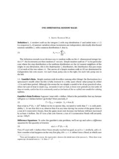
galton.uchicago.eduONE-DIMENSIONAL RANDOM WALKS 1. SIMPLE RANDOM WALK Definition 1. A random walk on the integers Z with step distribution F and initial state x 2Z is a sequenceSn of random variables whose increments are independent, identically distributed random variables ˘i with common distribution F, that is, (1) Sn =x + Xn i=1 ˘i. The definition extends in an obvious way …

Chapter 3 Formulation of FEM for Two-Dimensional Problems
users.metu.edu.tr3.1 Two-Dimensional FEM Formulation Many details of 1D and 2D formulations are the same. To demonstrate how a 2D formulation works well use the following steady, AD equation ⃗ in where ⃗ is the known velocity field, is the known and constant conductivity, is the known force ...

THREE DIMENSIONAL GEOMETRY - NCERT
www.ncert.nic.inTHREE DIMENSIONAL GEOMETRY 465 Hence, from (1), the d.c.’s of the line are 2 22 2 22 2 22, , a b c l m n abc abc abc =± =± =± ++ ++ ++ where, depending on the desired sign of k, either a positive or a negative sign is to be taken for l, m and n. For any line, if a, b, c are direction ratios of a line, then ka, kb, kc; k ≠ 0 is also a set of direction ratios.
Two-Dimensional Conduction: Finite-Difference Equations ...
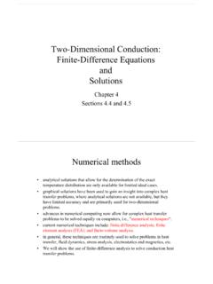
visualslope.comTwo-Dimensional Conduction: Finite-Difference Equations and Solutions Chapter 4 Sections 4.4 and 4.5 Numerical methods • analytical solutions that allow for the determination of the exact temperature distribution are only available for limited ideal cases. • graphical solutions have been used to gain an insight into complex heat

Reciprocal Space and Brillouin Zones in Two and Three ...
www.chem.tamu.eduThe two-dimensional square lattice is even simpler. The two lattice vectors a and b are equal in length and separated by a 90˚ angle. The reciprocal lattice basis vectors a* and b* are respectively perpendicular to a and b, and obviously make a 90˚ angle to each other. The reciprocal lattice points generated by these basis vectors is also