ELEMENTARY DIFFERENTIAL EQUATIONS
Chapter 8 Laplace Transforms 8.1 Introduction to the Laplace Transform 394 8.2 The Inverse Laplace Transform 406 8.3 Solution ofInitial Value Problems 414 8.4 The Unit Step Function 421 8.5 Constant Coefficient Equationswith Piecewise Continuous Forcing Functions 431 8.6 Convolution 441 8.7 Constant Cofficient Equationswith Impulses 453
Download ELEMENTARY DIFFERENTIAL EQUATIONS

Information
Domain:
Source:
Link to this page:
Documents from same domain
Probability, Statistics, and Stochastic Processes
ramanujan.math.trinity.eduProbability, Statistics, and Stochastic Processes Peter Olofsson Mikael Andersson A Wiley-Interscience Publication JOHN WILEY & SONS, INC. New York / Chichester / Weinheim / Brisbane / Singapore / Toronto
THE METHOD OF LAGRANGE MULTIPLIERS - Trinity …
ramanujan.math.trinity.eduTHE METHOD OF LAGRANGE MULTIPLIERS William F. Trench Andrew G. Cowles Distinguished Professor Emeritus Department of Mathematics Trinity University
INTRODUCTION TO REAL ANALYSIS - Trinity …
ramanujan.math.trinity.eduINTRODUCTION TO REAL ANALYSIS William F. Trench AndrewG. Cowles Distinguished Professor Emeritus Departmentof Mathematics Trinity University San Antonio, Texas, USA
Improper Integrals - Trinity University
ramanujan.math.trinity.eduThat’s the easy implication. For the converse, now suppose the stated Cauchy criterion holds. For natural numbers n alet a n = Z n a f(x)dx: Let …
STUDENT SOLUTIONS MANUAL FOR …
ramanujan.math.trinity.eduSTUDENT SOLUTIONS MANUAL FOR ELEMENTARY DIFFERENTIAL EQUATIONS AND ELEMENTARY DIFFERENTIAL EQUATIONS WITH BOUNDARY VALUE PROBLEMS William F. Trench Andrew G. Cowles Distinguished Professor Emeritus Department of Mathematics Trinity University San Antonio, Texas, USA
ELEMENTARY DIFFERENTIAL EQUATIONS
ramanujan.math.trinity.eduPreface Elementary Differential Equations with Boundary Value Problems is written for students in science, en-gineering,and mathematics whohave completed calculus throughpartialdifferentiation.
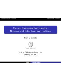
The one dimensional heat equation: Neumann and …
ramanujan.math.trinity.eduNeumann Boundary Conditions Robin Boundary Conditions Remarks At any given time, the average temperature in the bar is u(t) = 1 L Z L 0 u(x,t)dx. In the case of Neumann boundary conditions, one has u(t) = a 0 = f. That is, the average temperature is constant and is equal to the initial average temperature.
The two dimensional wave equation - Trinity University
ramanujan.math.trinity.eduThe 2D wave equation Separation of variables Superposition Examples Representability The question of whether or not a given function is equal to a double Fourier series is partially answered by the following result. Theorem If f(x,y) is a C2 function on the rectangle [0,a] ×[0,b], then
Introduction to Sturm-Liouville Theory - Trinity University
ramanujan.math.trinity.eduOrthogonality Sturm-Liouville problems Eigenvalues and eigenfunctions Inner products with weight functions Suppose that w(x) is a nonnegative function on [a,b].
The Chinese Remainder Theorem - ramanujan.math.trinity.edu
ramanujan.math.trinity.eduThe Chinese remainder theorem (CRT) asserts that there is a unique class a+ NZ so that xsolves the system (2) if and only if x2a+ NZ, i.e. x a(mod N). Thus the system (2) is equivalent to a single congruence modulo N. Although we only proved one implication, one can actually show that the …
Related documents

ELECTRONICS and CIRCUIT ANALYSIS using MATLAB
ee.hacettepe.edu.trInverse Laplace Transform 6.7 Magnitude and Phase Response of an RLC Circuit CHAPTER SEVEN TWO-PORT NETWORKS EXAMPLE DESCRIPTION 7.1 z-parameters of T-Network 7.2 y-parameters of Pi-Network 7.3 y-parameters of Field Effect Transistor 7.4 h-parameters of Bipolar Junction Transistor 7.5 Transmission Parameters of a Simple Impedance Network 7.6
AnIntroductionto StatisticalSignalProcessing
ee.stanford.eduLaplace argued to the effect that given complete knowledge of the physics of an ... and transform theory and applica-Preface xi tions. Detailed proofs are presented only when within the scope of this background. These simple proofs, however, often provide the groundwork for “handwaving” jus- ... examples, and problems. The
The Inverse Laplace Transform
howellkb.uah.edu530 The Inverse Laplace Transform 26.2 Linearity and Using Partial Fractions Linearity of the Inverse Transform The fact that the inverse Laplace transform is linear follows immediately from the linearity of the Laplace transform. To see that, let us consider L−1[αF(s)+βG(s)] where α and β are
Laplace Transform: Examples - Stanford University
math.stanford.eduLaplace Transform: Examples Def: Given a function f(t) de ned for t>0. Its Laplace transform is the function, denoted F(s) = Lffg(s), de ned by: F(s) = Lffg(s) = Z 1 0 e stf(t)dt: (Issue: The Laplace transform is an improper integral. So, does it always exist? i.e.: Is the function F(s) always nite?
Laplace Transform solved problems - Univerzita Karlova
matematika.cuni.czLaplace transform for both sides of the given equation. For particular functions we use tables of the Laplace transforms and obtain s(sY(s) y(0)) D(y)(0) = 1 s 1 s2 From this equation we solve Y(s) s3 y(0) + D(y)(0)s2 + s 1 s4 and invert it using the inverse Laplace transform and the same tables again and
SC505 STOCHASTIC PROCESSES Class Notes
www.mit.eduSC505 STOCHASTIC PROCESSES Class Notes c Prof. D. Castanon~ & Prof. W. Clem Karl Dept. of Electrical and Computer Engineering Boston University College of Engineering
PARTIAL DIFFERENTIAL EQUATIONS
web.math.ucsb.eduu(x;y) which satis es (1.1) for all values of the variables xand y. Some examples of PDEs (of physical signi cance) are: u x+ u y= 0 transport equation (1.2) u t+ uu x= 0 inviscid Burger’s equation (1.3) u xx+ u yy= 0 Laplace’s equation (1.4) u tt u xx= 0 wave equation (1.5) u t u xx= 0 heat equation (1.6) u t+ uu x+ u xxx= 0 KdV equation ...

18.03SCF11 text: Delta Functions: Unit Impulse
ocw.mit.edu4. Examples of integration Properties (3) and (2) show that δ(t) is very easy to integrate, as the following examples show: 5 Example 1. 7et2 cos(t)δ(t) dt = 7. All we had to do was evaluate the integrand at t = −5 0. 5 Example 2. 7et2 cos(t)δ(t − 2) dt = 7e4 cos(2). All we had to do was −5 evaluate the integrand at t = 2. 1
Basics of Signals and Systems - Univr
www.di.univr.it– Laplace Transform ! Basics – Z-Transform ! Basics Applications in the domain of Bioinformatics 4 . Gloria Menegaz What is a signal? • A signal is a set of information of data ... – Examples: signals defined through a mathematical function or graph • …

Chapter 7: The z-Transform
twins.ee.nctu.edu.twConvergence of Laplace Transform 7 z-transform is the DTFT of x[n]r n A necessary condition for convergence of the z-transform is the absolute summability of x[n]r n: The range of r for which the z-transform converges is termed the region of convergence (ROC). Convergence example: 1.