Search results with tag "Lagrange"

A Student’s Guide to Lagrangians and Hamiltonians
ppc.inr.ac.ruequations 70 3.2 Hamilton’s principle 73 3.3 Derivation of Lagrange’s equations 75 3.4 Generalization to many coordinates 75 3.5 Constraints and Lagrange’s λ-method 77 3.6 Non-holonomic constraints 81 3.7 Virtual work 83 3.7.1 Physical interpretation of the Lagrange multipliers 84 3.8 The invariance of the Lagrange equations 86 3.9 ...

Lecture L20 - Energy Methods: Lagrange’s
ocw.mit.eduSimple Pendulum by Lagrange’s Equations We first apply Lagrange’s equation to derive the equations of motion of a simple pendulum in polar coor dinates. This is a one degree of freedom system. However, it is convenient for later analysis of the double pendulum, to begin by describing the position of the mass point m 1 with cartesian ...
The Euler-Lagrange equation - KAIST
mathsci.kaist.ac.krNote that the Euler-Lagrange equation is only a necessary condition for the existence of an extremum (see the remark following Theorem 1.4.2). However, in many cases, the Euler-Lagrange equation by itself is enough to give a complete solution of the problem. In fact, the existence of an extremum is sometimes clear from the context of the problem.

Formule de Taylor-Lagrange - Claude Bernard University …
licence-math.univ-lyon1.frl’ordre 3, et écrire cette formule. Allez à : Correction exercice 1 Exercice 2. Soit un réel strictement positif. 1. Ecrire la formule de Taylor-Lagrange pour la fonction cosinus hyperbolique, sur l’intervalle [0, ], avec le reste à l’ordre 5. 2. Montrer que 0 Qch( )−1− 2 2! − 4 4! Q 5 5! sh( ) 3. En déduire que : 433 384 Qch(1 ...

LECTURE 3 LAGRANGE INTERPOLATION - University of …
coast.nd.eduCE30125 - Lecture 3 p. 3.1 LECTURE 3 LAGRANGE INTERPOLATION • Fit points with an degree polynomial • = exact function of which only discrete values are known and used to estab-

Extremos Restringidos (Multiplicadores de Lagrange)
sistemas.fciencias.unam.mxExtremos Restringidos (Multiplicadores de Lagrange) Dada la curva en el plano (x−h)2 a 2 (y−k)2 b = 1. Esta es una elipse con centro en (h,k) y queremos encontrar qu´e punto de esta elipse se encuentra m´as cercano al origen y que punto se encuentra
Chapter 2 Lagrange’s and Hamilton’s Equations
www.physics.rutgers.eduChapter 2 Lagrange’s and Hamilton’s Equations In this chapter, we consider two reformulations of Newtonian mechanics, the Lagrangian and the Hamiltonian formalism. The rst is naturally associated with con guration space, extended by time, while the latter is the natural description for working in phase space.

CSIR-UGC National Eligibility Test (NET) for Junior ...
www.csirhrdg.res.inRunge-Kutta methods. Calculus of Variations: Variation of a functional, Euler-Lagrange equation, Necessary and sufficient conditions for extrema.

Chapter 7 Hamilton's Principle - Lagrangian and ...
teacher.pas.rochester.eduPhysics 235 Chapter 7 - 4 - When we use the Lagrange's equations to describe the evolution of a system, we must recognize that these equations are only correct of the following conditions are met: 1. the force acting on the system, except the forces of constraint, must be derivable from one or more potentials.
THE METHOD OF LAGRANGE MULTIPLIERS - Trinity University
ramanujan.math.trinity.eduTrinity University San Antonio, Texas, USA wtrench@trinity.edu This is a supplement to the author’s Introductionto Real Analysis. It has been judged to meet the evaluation criteria set by the Editorial Board of the American Institute of Mathematics in connection with the Institute’s Open Textbook Initiative.
Mathematical Tools for Physics - Miami
www.physics.miami.eduDeriving Taylor Series Convergence Series of Series Power series, two variables Stirling’s Approximation Useful Tricks Di raction Checking Results 3 Complex Algebra 52 ... Lagrange Multipliers Solid Angle Rainbow 9 Vector Calculus 1 213 Fluid Flow Vector Derivatives Computing the divergence Integral Representation of Curl

Automatisation d’un poste de tri - Page Redirection
perso-laris.univ-angers.frQUEVREUX RINEAU LE TEXIER Projet M1 IAIE Poste de tri de colis automatisé Remerciements Nous tenons à remercier MM LAHAYE, LAGRANGE et …

Chapter 5: Numerical Integration and Differentiation
www.ece.mcmaster.caThis is to use a third-order Lagrange polynomial to fit to four points of f(x) ... 6480 f(4)(») where » is between a and b. 12. 3 Integration of Equations Newton-Cotes algorithms for equations Compare the following two Pseudocodes for multiple applications of the trape-zoidal rule. Pseudocode 1: Algorithm for multiple applications of the ...

Chapter7 Lagrangian and Hamiltonian Mechanics
bcas.du.ac.inequations of motion for small angle oscillations using Lagrange’s equations. Fig. 7.1 7.13 Use Hamilton’s equations to obtain the equations of motion of a uniform heavy rod of mass M and length 2a turning about one end which isfixed. 7.14 A one-dimensional harmonic oscillator has Hamiltonian H = 1 2 p 2 + 1 2ω 2q2. Write down Hamiltonian ...
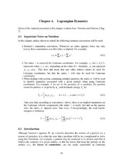
Chapter 4. Lagrangian Dynamics
physics.uwo.caHamilton’s Principle, from which the equations of motion will be derived. These equations are called Lagrange’s equations. Although the method based on Hamilton’s Principle does not constitute in itself a new physical theory, it is probably justified to say that it is more fundamental that Newton’s equations.

8.09(F14) Chapter 4: Canonical Transformations, Hamilton ...
ocw.mit.eduChapter 4 Canonical Transformations, Hamilton-Jacobi Equations, and ... Recall the the Euler-Lagrange equations are invariant when: 60. CHAPTER 4. CANONICAL TRANSFORMATIONS, HAMILTON-JACOBI ... where the Hamilton’s equations for the evolution of the canonical variables (q;p) are satis ed: @H q_ i= @H and p_ i = @p. i
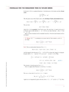
FORMULAS FOR THE REMAINDER TERM IN TAYLOR SERIES
www.stewartcalculus.comThe formula for the remainder term in Theorem 4 is called Lagrange’s form of the remainder term. Notice that this expression is very similar to the terms in the Taylor series except that is evaluated at instead of at . All we can say about the number is that it lies somewhere between and .

The Hamiltonian method
scholar.harvard.eduXV-2 CHAPTER 15. THE HAMILTONIAN METHOD ilarities between the Hamiltonian and the energy, and then in Section 15.2 we’ll rigorously deflne the Hamiltonian and derive Hamilton’s equations, which are the equations that take the place of Newton’s laws and the Euler-Lagrange equations.

The Lagrangian Method - Harvard University
scholar.harvard.edu6.1 The Euler-Lagrange equations Here is the procedure. Consider the following seemingly silly combination of the kinetic and potential energies (T and V, respectively), L · T ¡V: (6.1) This is called the Lagrangian. Yes, there is a minus sign in the deflnition (a plus sign would simply give the total energy).
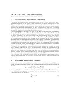
PHYS 7221 - The Three-Body Problem
www.phys.lsu.edu4 Lagrange’s Solution This case is realized when G = 0 and the equations for the si decouple. The three decoupled equations have the two-body form whose solutions are ellipses for bound cases. The condition for G = 0 is that s1 = s2 = s3, in other words the particles sit at the vertexes of an equilateral triangle

Higher-Order Derivatives and Taylor’s Formula in Several ...
sites.math.washington.eduHigher-Order Derivatives and Taylor’s Formula in Several Variables G. B. Folland ... can be obtained from the Lagrange or integral formulas for remainders, applied to g. It is usually preferable, however, to rewrite (2) and the accompanying formulas for the

Real Analysis Math 125A, Fall 2012 Final Solutions 1. R
www.math.ucdavis.edukth Taylor coefficient of f(x) = ex at zero is ak = f(k)(0) k! = 1 k!, and Pn(x) = ∑n k=0 1 k! xk = 1+x+ 1 2! x2 +···+ 1 n! xn. • (b) The expression for the Lagrange remainder is Rn(x) = 1 (n+1)! f(n+1)(ξ)xn+1 = 1 (n+1)! e˘ xn+1 for some ξ strictly between 0 and x. • (c) For n = 1, we get ex = 1+x+ 1 2 e˘x2. Since e˘ > 0, it ...
Lagrange Multipliers - Illinois Institute of Technology
web.iit.eduLagrange method is used for maximizing or minimizing a general function f(x,y,z) subject to a constraint (or side condition) of the form g(x,y,z) =k. Assumptions made: the extreme values exist ∇g≠0 Then there is a number λ such that ∇ f(x 0,y 0,z 0) =λ ∇ g(x 0,y 0,z 0) and λ is called the Lagrange multiplier. ….

Lagrange’s Method - University of California, San Diego
maecourses.ucsd.eduLagrange’s Method application to the vibration analysis of a flexible structure ∗ R.A. de Callafon University of California, San Diego 9500 Gilman Dr. La Jolla, CA 92093-0411 callafon@ucsd.edu Abstract This handout gives a short overview of the formulation of the equations of motion for a flexible system using Lagrange’s equations ...

Lagrange-Ansatz - matp.de
matp.deLagrange-Ansatz 1Motivation Die Präferenzen von Otto Optimal bezüglich Gut 1 (Aktien von BMW) und Gut 2 (Aktien von VW) lassen sich mit Hilfe folgender Nutzenfunktion beschreiben: u(x 1;x 2) = 400x 1x22 Otto Optimal verdient 3000 Euro im Monat.

Lagrange Interpolating Polynomials - University of Florida
people.clas.ufl.eduLagrange Interpolating Polynomials James Keesling ... 5 Taylor polynomials Occasionally one may want other conditions on a polynomial other than tting values at di erent points. The most important is determining the polynomial that has a certain set of derivatives at a point. In this case the point is taken to be x

Lagrange Multipliers and the Karush-Kuhn-Tucker …
www.csc.kth.seIf x corresponds to a constrained local minimum then Case 1: Unconstrained local minimum occurs in the feasible region. 1 g(x ) <0 2 r x f(x ) = 0 3 r xx f(x ) is a positive semi-de nite matrix. Case 2: Unconstrained local minimum lies outside the feasible region. 1 g(x ) = 0 2 r xf(x ) = rg(x ) with >0 3 ytr xx L(x )y 0 for all y orthogonal to ...

Lagrange’s Theorem: Statement and Proof
www.stolaf.eduLemma 1. If Gis a group with subgroup H, then there is a one to one correspondence between H and any coset of H. Proof. Let Cbe a left coset of Hin G. Then there is a g2Gsuch that C= g H.1 De ne f: H!Cby f(x) = gx. 1. fis one to one. If x 1 6= x 2, then as Ghas cancellation, gx 1 6= gx 2. Hence, f(x 1) 6= f(x 2). 2. fis onto.
Similar queries
Equations, 2 Hamilton, Lagrange, S equations, Lagrange equations, Formule, Taylor-Lagrange, LAGRANGE INTERPOLATION, Chapter 2 Lagrange’s and Hamilton’s Equations, Chapter, Euler-Lagrange, Hamilton, Trinity, Taylor, Chapter 4: Canonical Transformations, Hamilton, Chapter 4 Canonical Transformations, Hamilton-Jacobi Equations, and, CHAPTER 4. CANONICAL TRANSFORMATIONS, HAMILTON, FORMULAS FOR THE REMAINDER TERM IN TAYLOR SERIES, Hamiltonian, 2 CHAPTER, Lagrangian, Lagrange Multipliers and the Karush-Kuhn-Tucker, Local, Lagrange’s Theorem: Statement and Proof, Correspondence