ELEMENTARY DIFFERENTIAL EQUATIONS
Chapter 8 Laplace Transforms 8.1 Introduction to the Laplace Transform 394 8.2 The Inverse Laplace Transform 406 8.3 Solution ofInitial Value Problems 414 8.4 The Unit Step Function 421 8.5 Constant Coefficient Equationswith Piecewise Continuous Forcing Functions 431 8.6 Convolution 441 8.7 Constant Cofficient Equationswith Impulses 453
Download ELEMENTARY DIFFERENTIAL EQUATIONS

Information
Domain:
Source:
Link to this page:
Documents from same domain
Probability, Statistics, and Stochastic Processes
ramanujan.math.trinity.eduProbability, Statistics, and Stochastic Processes Peter Olofsson Mikael Andersson A Wiley-Interscience Publication JOHN WILEY & SONS, INC. New York / Chichester / Weinheim / Brisbane / Singapore / Toronto
THE METHOD OF LAGRANGE MULTIPLIERS - Trinity …
ramanujan.math.trinity.eduTHE METHOD OF LAGRANGE MULTIPLIERS William F. Trench Andrew G. Cowles Distinguished Professor Emeritus Department of Mathematics Trinity University
INTRODUCTION TO REAL ANALYSIS - Trinity …
ramanujan.math.trinity.eduINTRODUCTION TO REAL ANALYSIS William F. Trench AndrewG. Cowles Distinguished Professor Emeritus Departmentof Mathematics Trinity University San Antonio, Texas, USA
Improper Integrals - Trinity University
ramanujan.math.trinity.eduThat’s the easy implication. For the converse, now suppose the stated Cauchy criterion holds. For natural numbers n alet a n = Z n a f(x)dx: Let …
STUDENT SOLUTIONS MANUAL FOR …
ramanujan.math.trinity.eduSTUDENT SOLUTIONS MANUAL FOR ELEMENTARY DIFFERENTIAL EQUATIONS AND ELEMENTARY DIFFERENTIAL EQUATIONS WITH BOUNDARY VALUE PROBLEMS William F. Trench Andrew G. Cowles Distinguished Professor Emeritus Department of Mathematics Trinity University San Antonio, Texas, USA
ELEMENTARY DIFFERENTIAL EQUATIONS
ramanujan.math.trinity.eduPreface Elementary Differential Equations with Boundary Value Problems is written for students in science, en-gineering,and mathematics whohave completed calculus throughpartialdifferentiation.
The one dimensional heat equation: Neumann and …
ramanujan.math.trinity.eduNeumann Boundary Conditions Robin Boundary Conditions Remarks At any given time, the average temperature in the bar is u(t) = 1 L Z L 0 u(x,t)dx. In the case of Neumann boundary conditions, one has u(t) = a 0 = f. That is, the average temperature is constant and is equal to the initial average temperature.
The two dimensional wave equation - Trinity University
ramanujan.math.trinity.eduThe 2D wave equation Separation of variables Superposition Examples Representability The question of whether or not a given function is equal to a double Fourier series is partially answered by the following result. Theorem If f(x,y) is a C2 function on the rectangle [0,a] ×[0,b], then
Introduction to Sturm-Liouville Theory - Trinity University
ramanujan.math.trinity.eduOrthogonality Sturm-Liouville problems Eigenvalues and eigenfunctions Inner products with weight functions Suppose that w(x) is a nonnegative function on [a,b].
The Chinese Remainder Theorem - ramanujan.math.trinity.edu
ramanujan.math.trinity.eduThe Chinese remainder theorem (CRT) asserts that there is a unique class a+ NZ so that xsolves the system (2) if and only if x2a+ NZ, i.e. x a(mod N). Thus the system (2) is equivalent to a single congruence modulo N. Although we only proved one implication, one can actually show that the …
Related documents
Laplace Transform solved problems - cuni.cz
matematika.cuni.czUsing the Laplace transform nd the solution for the following equation @ @t y(t) = e( 3t) with initial conditions y(0) = 4 Dy(0) = 0 Hint. no hint Solution. We denote Y(s) = L(y)(t) the Laplace transform Y(s) of y(t). We perform the Laplace transform for both sides of the given equation. For particular functions we use tables of the Laplace ...
The Inverse Laplace Transform
howellkb.uah.edu532 The Inverse Laplace Transform! Example 26.5: In exercise25.1e on page 523, you found thatthe Laplacetransformof the solution to y′′ + 4y = 20e4t with y(0) = 3 and y′(0) = 12 is Y(s) = 3s2 −28 (s −4). s2 +4 The partial fraction expansion of this is Y(s) = 3s2 −28 (s − 4) s2 +4 A s − + Bs +C s2 +4 for some constants A, B and C .
1 Z-Transforms, Their Inverses Transfer or System Functions
web.eecs.umich.eduIf you don’t know what a Laplace transform is, you aren’t missing anything that will help you. The above three properties still hold, but computing X(z) now requires use of: ... Solution: Take the z-transforms of the difference equation and of the input. This yields Y(z) −2z−1Y(z) = z−1X(z)−z−2X(z); X(z) = z z −3

Chapter 13: The Laplace Transform in Circuit Analysis
jazapka.people.ysu.edusolution satisfied the given initial conditions and final behavior. ... Transfer Function: the s-domain ratio of the Laplace transform of the output (response) to the Laplace transform of the input (source) ℒ ℒ Example. Finding the transfer function of an RLC circuit If the voltage is the desired output: ...

Solving Differential Equations Using Simulink
people.uncw.eduJul 01, 2019 · related to the Laplace transform L Z t 0 f(t)dt = 1 s F(s), where F(s) is the Laplace transform of f(t). integrate dx dt, producing x(t). introduction to simulink 3 ... The solution shown in Figure 1.13 had a setting of 1 and that in Figure 1.16 …
TABLE OF INVERSE LAPLACE TRANSFORMS
webster.math.umbc.edufirst- and second-order equations, followed by Chapter 5 (the Laplace transform), Chapter 6 (systems), Chapter 8 (nonlinear equations), and part of Chapter 9 (partial differential equations). I generally spend a couple of days giving a rough overview of the omitted chapters: series solutions (Chapter 4) and difference equations (Chapter 7).
Solution of ODEs using Laplace Transforms - Queen's U
chemeng.queensu.caSolution of ODEs We can continue taking Laplace transforms and generate a catalogue of Laplace domain functions. The final aim is the solution of ordinary differential equations. Example Using Laplace Transform, solve Result

Lecture #7 Lagrange's Equations - MIT OpenCourseWare
ocw.mit.eduLaplace, Legendre (Newton 1643-1727) • Contributions o Calculus of variations ... Example: Work in polar coordinates, then transform to rectangular coordinates, e.g. sin cos ... Existence of constraints complicates the solution of the problem.
Section 7.4: Inverse Laplace Transform - University of Florida
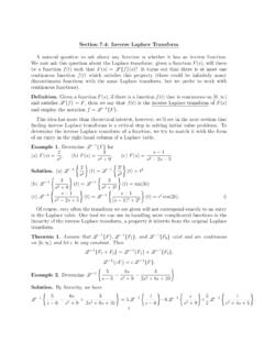
people.clas.ufl.edunding inverse Laplace transforms is a critical step in solving initial value problems. To determine the inverse Laplace transform of a function, we try to match it with the form of an entry in the right-hand column of a Laplace table. Example 1. Determine L 1fFgfor (a) F(s) = 2 s3, (b) F(s) = 3 s 2+ 9, (c) F(s) = s 1 s 2s+ 5. Solution. (a) L 21 ...

Convolution solutions (Sect. 6.6). Convolution of two ...
users.math.msu.eduI Laplace Transform of a convolution. I Impulse response solution. I Solution decomposition theorem. Laplace Transform of a convolution. Theorem (Laplace Transform) If f , g have well-defined Laplace Transforms L[f ], L[g], then L[f ∗ g] = L[f ] L[g]. Proof: The key step is to interchange two integrals. We start we the product of the Laplace ...