ERROR IN LINEAR INTERPOLATION

THE SECANT METHOD - University of Iowa

THE SECANT METHOD Newton’s method was based on using the line tangent to the curve of y = f(x), with the point of tangency (x 0;f(x 0)).When x 0 ˇ , the graph of the tangent line is approximately the same as the

  Methods, Ascent, The secant method

NUMERICALSOLUTIONOF ORDINARYDIFFERENTIAL …

The differential equations we consider in most of the book are of the form Y′(t) = f(t,Y(t)), where Y(t) is an unknown function that is being sought. The given function f(t,y) of two variables defines the differential equation, and exam ples are given in Chapter 1. This equation is called a first-order differential equation because it ...

  Differential

Lecture 1: The Euler characteristic

7 vertices, 9 edges, 2 faces. We wish to count: 3 vertices, 3 edges, 1 face. 6 vertices, 9 edges, 4 faces. Euler characteristic (simple form): = number of vertices – number of edges + number of faces Or in short-hand, = |V| - |E| + |F| where V = set of vertices E = set of edges ...

  Lecture, Characteristics, Vertices, Euler, Lecture 1, The euler characteristic

TRAPEZOIDAL METHOD: ERROR FORMULA

The corrected trapezoidal rule is illustrated in the following table. n I T n Ratio I CT n Ratio 2 5.319 3.552E 1 4 1.266 4.20 2.474E 2 14.4 8 3.118E 1 4.06 1.583E 3 15.6

  Rules

NUMERICAL STABILITY; IMPLICIT METHODS

The numerical methods studied in this chapter are both stable and convergent. All of these general results on stability and convergence are valid if the stepsize h is su ciently small. What is meant by this? ... 64E 4 5 2:83E+ 4 3:78E 3 3:97E 4 50 1 3:26E+ 0 1:06E+ 3 1:39E 4 3 1:08E+ 6 1:17E+ 15 8:25E 5 5 3:59E+ 11 1:28E+ 27 7:00E 5.

  Methods, Chapter, Stability, Numerical, Implicit, Numerical stability implicit methods

A quick example calculating the column space and the ...

Put A into echelon form and then into reduced echelon form: R 2 –R 1 R 2 R 3 + 2R 1 R 3 R 1 + 5R 2 R 1 R 2 /2 R 2 R 1 + 8R 3 ...

  Example, Quick, Reduced, Calculating, Space, Columns, Echelon, Quick example calculating the column space and, Reduced echelon

Runge-Kutta 4th Order Method for Ordinary Differential ...

Oct 13, 2010 · Runge-Kutta 4th order method is a numerical technique to solve ordinary differential used equation of the form . f (x, y), y(0) y 0 dx dy = = So only first order ordinary differential equations can be solved by using Rungethe -Kutta 4th order method. In other sections, we have discussed how Euler and Runge-Kutta methods are

  Runge, Kutta, Runge kutta

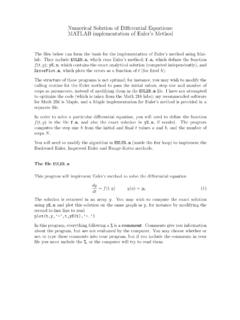
Numerical Solution of Differential Equations: MATLAB ...

Backward Euler, Improved Euler and Runge-Kutta methods. The file EULER.m This program will implement Euler’s method to solve the differential equation dy dt = f(t,y) y(a) = y 0 (1) The solution is returned in an array y. You may wish to compute the exact solution using yE.m and plot this solution on the same graph as y, for instance by ...

  Matlab, Runge

NUMERICALSOLUTIONOF ORDINARYDIFFERENTIAL …

9.1 Families of implicit Runge–Kutta methods 149 9.2 Stability of Runge–Kutta methods 154 9.3 Order reduction 156 9.4 Runge–Kutta methods for stiff equations in practice 160 Problems 161 10 Differential algebraic equations 163 10.1 Initial conditions and drift 165 10.2 DAEs as stiff differential equations 168

  Runge, Numericalsolutionof ordinarydifferential, Numericalsolutionof, Ordinarydifferential

Solving ODEs in Matlab - MIT

Runge-Kutta (4,5) formula *No precise definition of stiffness, but the main idea is that the equation includes some terms that can lead to rapid variation in the solution. [t,state] = ode45(@dstate,tspan,ICs,options) Defining an ODE function in an M-file

  Runge

Neural Ordinary Differential Equations

directly through a Runge-Kutta integrator, re-ferred to as RK-Net. Table1shows test error, number of parameters, and memory cost. Ldenotes the number of layers in the ResNet, and L~ is the number of function evaluations that the ODE solver requests in a single forward pass, which can be interpreted as an implicit number of layers. We find

  Runge

Quadratic Spline Example

The upward velocity of a rocket is given as a function of time in table below. Find the velocity and acceleration at t=16 seconds.

Textbook notes for Runge-Kutta 2nd Order Method for ...

Oct 13, 2010 · The Runge-Kutta 2nd order method is a numerical technique used to solve an ordinary differential equation of the form . f (x, y), y(0) y 0 dx dy = = Only first order ordinary differential equations can be solved by uthe Runge-Kutta 2nd sing order method. In other sections, we will discuss how the Euler and Runge-Kutta methods are

  Runge, Kutta, Runge kutta

Chapter 6: Molecular Dynamics - Missouri S&T

•Math simpler than two Runge-Kutta algorithms required for a 2nd order ODE Note: velocities do not show up! If velocities are desired: Physics 5403: Computational Physics - Chapter 6: Molecular Dynamics 19 Disadvantages: •Accuracy of velocities is only O ...

  Runge

Jeffrey R. Chasnov

Chapter 1 IEEE Arithmetic 1.1Definitions Bit = 0 or 1 Byte = 8 bits Word = Reals: 4 bytes (single precision) 8 bytes (double precision) = Integers: 1, 2, 4, or 8 byte signed

  Jeffrey, Jeffrey r, Chasnov

Quantum Physics III Chapter 2: Hydrogen Fine Structure

n. This degeneracy explained by the existence of a conserved quantum Runge-Lenz vector. For a given nthe states with various ℓ’s correspond, in the semiclassical picture, to orbits of different eccentricity but the same semi-major axis. The orbit with ℓ= 0 is the most eccentric one and the orbit with maximum ℓ= n− 1 is the most ...

  Runge