Finite Difference Method for Solving Differential Equations
matrix form as . 2 × × = − − − − 0 9.375 10 9.375 10 0 0 0 0 1 0032020 .0016 0.0016 0.003202 0.0016 0 1 0 4 4 4 3 1 y y y y. The above equations have a coefficient matrix that is tridiagonal (we can use Thomas’ algorithm to solve the equations) and is also strictly diagonally dominant (convergence is guaranteed if we use iterative ...
Download Finite Difference Method for Solving Differential Equations

Information
Domain:
Source:
Link to this page:
Documents from same domain

Chapter 01.03 Sources of Error - MATH FOR COLLEGE
mathforcollege.com01.03.1 Chapter 01.03 Sources of Error After reading this chapter, you should be able to: 1. know that there are two inherent sources of error in numerical methods – round-

Runge-Kutta 4th Order Method for Ordinary …
mathforcollege.com08.04.1 Chapter 08.04 Runge-Kutta 4th Order Method for Ordinary Differential Equations . After reading this chapter, you should be able to . 1. develop Runge-Kutta 4th order method for solving ordinary differential equations,

Simpson 3/8 Rule for Integration - MATH FOR …
mathforcollege.comIn a similar fashion, Simpson rule for integration can be derived by 3/8 approximating the given function
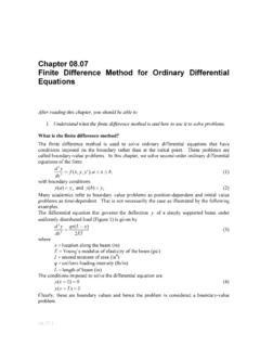
Finite Difference Method for Solving Differential …
mathforcollege.com08.07.1 . Chapter 08.07 Finite Difference Method for Ordinary Differential Equations . After reading this chapter, you should be able to . 1. Understand what the finite difference method is and how to use it to solve problems.

Chapter 04.08 Gauss-Seidel Method
mathforcollege.comusing the Gauss-Seidel method. Assume an initial guess of the solution as = 5 2 1
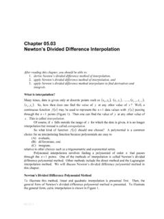
Chapter 05.03 Newton’s Divided Difference Interpolation
mathforcollege.comNewton’s Divided Difference Interpolation 05.03.3 Figure 2 Linear interpolation. Example 1 The upward velocity of a rocket is given as a function of time in Table 1 (Figure 3).

False-Position Method of Solving a Nonlinear Equation
mathforcollege.com03.06.1 . Chapter 03.06 False-Position Method of Solving a Nonlinear Equation . After reading this chapter, you should be able to . 1. follow the algorithm of the false-position method of solving a nonlinear equation,
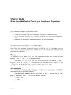
Bisection Method of Solving Nonlinear Equations: General ...
mathforcollege.comOne of the first numerical methods developed to find the root of a nonlinear equation . f (x) =0 was the bisection method (also called binary-search method). The method is based on the following theorem. Theorem. An equation. f (x) =0, where f (x) is a real continuous function, has at least one root between . x and . x. u. if f (x ) f (x. u ...
Runge-Kutta 4th Order Method for Ordinary Differential ...
mathforcollege.comOct 13, 2010 · 08.04.1 Chapter 08.04 Runge-Kutta 4th Order Method for Ordinary Differential Equations . After reading this chapter, you should be able to . 1. develop Runge-Kutta 4th order method for solving ordinary differential equations, 2. find the effect size of step size has on the solution, 3. know the formulas for other versions of the Runge-Kutta 4th order method
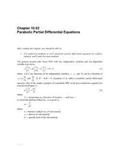
Chapter 10.02 Parabolic Partial Differential Equations
mathforcollege.comParabolic Partial Differential Equations . After reading this chapter, you should be able to: 1. Use numerical methods to solve parabolic partial differential eqplicit, uations by ex implicit, and Crank-Nicolson methods. The general second order linear PDE with two independent variables and one dependent variable is given by . 0. 2 2 2 2 2 ...
Related documents
Alternating Direction Method of Multipliers
web.stanford.eduproximal point algorithm (Rockafellar 1976) ... tridiagonal matrix) Examples 33. Outline Dual decomposition Method of multipliers Alternating direction method of multipliers Common patterns Examples Consensus and exchange Conclusions Consensusandexchange 34. …

Iterative Methods for Sparse Linear Systems
web.stanford.eduIterative methods for solving general, large sparse linear systems have been gaining popularity in many areas of scientific computing. Until recently, direct solution methods

Numerical Recipes in C - grad.hr
www.grad.hr2.4 Tridiagonal and Band Diagonal Systems of Equations 50 2.5 Iterative Improvement of a Solution to Linear Equations 55 2.6 Singular Value Decomposition 59 2.7 Sparse Linear Systems 71 2.8 Vandermonde Matrices and Toeplitz Matrices 90 2.9 Cholesky Decomposition 96 2.10 QR Decomposition 98 2.11 Is Matrix Inversion an N3 Process? 102

Tridiagonal Matrices: Thomas Algorithm
www.industrial-maths.comTridiagonal Matrices: Thomas Algorithm W. T. Lee∗ MS6021, Scientific Computation, University of Limerick The Thomas algorithm is an efficient way of solving tridiagonal matrix syste ms. It is based on LU decompo-sition in which the matrix system Mx =r is rewritten as LUx =r where L is a lower triangular matrix and U is an upper triangular ...