FINITE ELEMENT METHOD
1. Finite Difference Method (FDM) 2. Finite Volume Method (FVM) 3. Finite Element Method (FEM) 4. Boundary Element Method (BEM) 5. Spectral Method 6. Perturbation Method (especially useful if the equation contains a small parameter) 1.1 Finite Difference Method The finite difference method is the easiest method to understand and apply.
Download FINITE ELEMENT METHOD

Information
Domain:
Source:
Link to this page:
Documents from same domain

FORMAT FOR PREPARATION OF PROJECT REPORT
www.iist.ac.inFORMAT FOR PREPARING THE INTERNSHIP PROJECT REPORT ... 3.1 Cover Page & Title Page – A specimen copy of the Cover page & Title page of the ... as per the format in Appendix 2. The certificate shall carry the supervisor‟s signature and HoD's signature fro projects done in IIST and signatures of equivalent people if it is done outside IIST.

Conservation Equations of Fluid Dynamics
www.iist.ac.inConservation Equations of Fluid Dynamics A. Salih Department of Aerospace Engineering Indian Institute of Space Science and Technology, Thiruvananthapuram { February 2011 {This is a summary of conservation equations (continuity, Navier{Stokes, and energy) that govern the ow of a Newtonian uid.

Delta Function and Heaviside Function - IIST
www.iist.ac.inIf the delta function is acting at the origin, i.e., if a =0, the regularized delta function defined by (15) becomes δε(x)= 1 2ε 1+cos πx ε if −ε<x <ε, 0 otherwise. (17) Another example of regularized delta function is a sequence of bell-shaped pulses defined as δk(x−a)= 1 k √ 2π e− 1 2(x−a k) 2 (18) where k is a parameter.

Streamfunction-Vorticity Formulation
www.iist.ac.inThe relation connecting the streamfunction and vorticity (6) is listed below: ¶2y ¶x2 ¶2y ¶y2 = w (15) Equations (14) and (15) form the system PDEs for streamfunction-vorticity formulation.

Method of Characteristics - Home | IIST
www.iist.ac.inThe method of characteristics is a technique for solving hyperbolic partial differential equa-tions (PDE). Typically the method applies to first-order equations, although it is valid for any 3. hyperbolic-type PDEs. The method involves the determination of special curves, called char-

Kelvin–Helmholtz Instability - IIST
www.iist.ac.inkinematic boundary condition which states that the interface moves up and down with a velocity ... complex wave speed. Note that hˆ is the original amplitude of the interface displacement and is a constant. It speci es the size of all perturbed quantities. When c

FORMAT FOR PREPARATION OF PROJECT REPORT
www.iist.ac.in3.2 Bonafide Certificate – The Bonafide Certificate shall be in double line spacing Times New Roman using Font Style and Font Size 14, as per the format in Appendix 2. The certificate shall carry the supervisor‟s signature and HoD's signature fro projects done in IIST and signatures of equivalent people if it is done outside IIST.
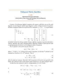
Tridiagonal Matrix Algorithm - Indian Institute of Space ...
www.iist.ac.inThomas’ algorithm, also called TriDiagonal Matrix Algorithm (TDMA) is essentially the result of applying gaussian elimination to the tridiagonal system of equations. The ith equation in the system may be written as a iu i 1 + b iu i + c iu i+1 = d i (2) where a 1 =0 and c N =0. Looking at the system of equations, we see that ith unknown can be

Second-Order Wave Equation - Indian Institute of Space ...
www.iist.ac.inthe domain is infinite. In this method, a canonical form of the wave equation (3) is first obtained using a suitable transformation. The canonical form enable us to easily integrate the equation to obtain the general solution. Below we give a brief description of the solution method. We can factor the linear differential operators of (3) to ...
Related documents
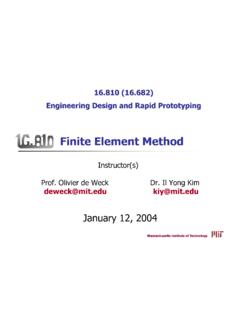
Finite Element Method
web.mit.edu16.810 (16.682) 2 Plan for Today FEM Lecture (ca. 50 min) FEM fundamental concepts, analysis procedure Errors, Mistakes, and Accuracy Cosmos Introduction (ca. 30 min) Follow along step-by-step Conduct FEA of your part (ca. 90 min) Work in teams of two First conduct an analysis of your CAD design You are free to make modifications to your original model
An Introduction to Computational Fluid Dynamics
www2.mie.utoronto.caflow solver: (i) finite difference method; (ii) finite element method, (iii) finite volume method, and (iv) spectral method. (3) A post-processor, which is used to massage the data and show the results in graphical and easy to read format. In this chapter we are mainly concerned with the flow solver part of CFD. This chapter is

An introduction to optimization on smooth manifolds
sma.epfl.ch10.6 Finite difference approximation of the Hessian 268 10.7 Tensor fields and their covariant differentiation 271 10.8 Notes and references 278 11 Geodesic convexity 283 11.1 Convex sets and functions 283 11.2 Geodesically convex sets and functions 286 11.3 Differentiable geodesically convex functions 290 11.4 Positive reals and geometric ...

Chap-5 (8th Nov.) - NCERT
ncert.nic.inHere the difference of any two consecutive terms in each case is 3. So, the given list is an AP whose first term a is 6 and common difference d is 3. For the list of numbers : 6, 3, 0, – 3, . . ., a 2 – a 1 = 3 – 6 = – 3 a 3 – a 2 = 0 – 3 = – 3 a 4 – a 3 = –3 – 0 = –3 Similarly this is also an AP whose first term is 6 and ...