Joint and Marginal Distributions
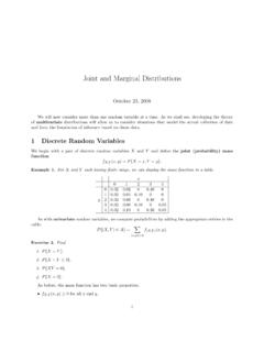
The marginal mass functions for the example above are x f X(x) 0 0.10 1 0.30 2 0.20 3 0.30 4 0.10 y f Y (y) 0 0.14 1 0.16 2 0.18 3 0.25 4 0.27 Exercise 3. Give two pairs of random variables with different joint mass functions but the same marginal mass functions.
Download Joint and Marginal Distributions

Information
Domain:
Source:
Link to this page:
Documents from same domain
Chapter 6 Importance sampling
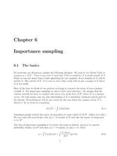
www.math.arizona.edurandom variable we want to compute the mean of is of the form f(X~) where X~ is a random vector. We will assume that the joint distribution of X~ is absolutely continous and let p(~x) be the density. (Everything we will do also works for the case where the random vector X~ is discrete.) So we focus on computing Ef(X~) = Z f(~x)p(~x)dx (6.1)
1 Sufficient statistics
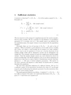
www.math.arizona.educonditional distribution. But then his random sample has the same distri-bution as a random sample drawn from the population (with its unknown value of θ). So statistician B can use his random sample X0 1,···,X0 n to com-pute whatever statistician A computes using his random sample X1,···,Xn, and he will (on average) do as well as ...
A Conditional expectation
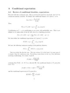
www.math.arizona.eduThe partition theorem says that if Bn is a partition of the sample space then E[X] = X n E[XjBn]P(Bn) Now suppose that X and Y are discrete RV’s. If y is in the range of Y then Y = y is a event with nonzero probability, so we can use it as the B in the above.
Method of Moments - University of Arizona
www.math.arizona.eduThe muon is an elementary particle with an electric charge of 1 and a spin (an intrinsic angular momentum) of 1/2. It is an unstable subatomic particle with a mean lifetime of 2.2 µs. Muons have a mass of about 200 times the mass of an electron. Since the muon’s charge and spin are the same as the electron, a muon can be

Topic 15 Maximum Likelihood Estimation
www.math.arizona.eduMaximum Likelihood Estimation Multidimensional Estimation 1/10. Fisher Information Example Outline Fisher Information Example Distribution of Fitness E ects ... To obtain the maximum likelihood estimate for the gamma family of random variables, write the likelihood L( ; jx) = ( ) x 1 1 e x1 ( ) x 1 n e xn = ( ) n (x 1x 2 x
Maximum Likelihood Estimation - University of Arizona
www.math.arizona.eduIntroduction to the Science of Statistics Maximum Likelihood Estimation 0.2 0.3 0.4 0.5 0.6 0.7 0.0e+00 5.0e-07 1.0e-06 1.5e-06 p l 0.2 0.3 0.4 0.5 0.6 0.7
Topic 15: Maximum Likelihood Estimation
www.math.arizona.eduIntroduction to Statistical Methodology Maximum Likelihood Estimation Exercise 3. Check that this is a maximum. Thus, p^(x) = x: In this case the maximum likelihood estimator is also unbiased. Example 4 (Normal data). Maximum likelihood estimation can be applied to a vector valued parameter. For a simple
Innovative Methods of Teaching - University of Arizona
www.math.arizona.eduThe reason being that martyr is engaged in defense work while an alim (scholar) builds individuals and nations along positive lines. In this way he bestows a real life to the world. “Education is the manifestation of perfection already in man” – (Swami Vivekananda)
Probability Theory - University of Arizona
www.math.arizona.eduProbability Theory December 12, 2006 Contents 1 Probability Measures, Random Variables, and Expectation 3 ... Definition 1.18. Let f : (S,S) → (T,T ) be a function between measure spaces, then f is called measurable if f−1(B) ∈ S for every B ∈ T . (1.6) If (S,S) has a probability measure, then f is called a random variable.

Interval Estimation - University of Arizona
www.math.arizona.edulikelihood, and evaluate the quality of the estimator by evaluating the bias and the variance of the estimator. Often, we know more about the distribution of the estimator and this allows us to take a more comprehensive statement about the estimation procedure. Interval estimation is an alternative to the variety of techniques we have examined.
Related documents
Density of States - gatech.edu
alan.ece.gatech.eduDerivation of Density of States (2D) Thus, where The solutions to the wave equation where V(x) = 0 are sine and cosine functions Since the wave function equals zero at the infinite barriers of the well, only the sine function is valid. Thus, only the following values are possible for the wave number (k): 2 2 2 2 2 2 1 1 k y k x y x = − ∂ ...

Integral Calculus Formula Sheet
mslc.osu.eduAlgebraic Functions (xx x3,5,1/, etc) Trig Functions (sin(5 ),tan( ),xxetc) dv Exponential Functions (e33xx,5 ,etc) Functions that appear at the top of the list are more like to be u, functions at the bottom of the list are more like to be dv. Trig Integrals:

Power Spectral Density - MIT OpenCourseWare
ocw.mit.edu184 Chapter 10 Power Spectral Density where Sxx(jω) is the CTFT of the autocorrelation function Rxx(τ).Furthermore, when x(t) is ergodic in correlation, so that time averages and ensemble averages are equal in correlation computations, then (10.1) also represents the time-average

Wave Functions - Weber State University
physics.weber.edudensity, we use sinusoidal functions that are out of phase by a quarter cycle (ˇ=2, or 90 ), so that one component is large in magnitude where the other is zero and vice-versa. And to distinguish left-moving from right-moving particles, we associate
2 Heat Equation - Stanford University
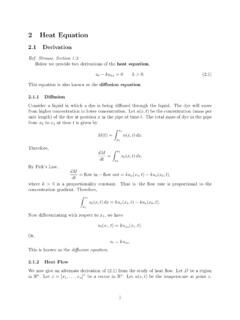
web.stanford.edutime t, and let H(t) be the total amount of heat (in calories) contained in D.Let c be the specific heat of the material and ‰ its density (mass per unit volume). Then H(t) = Z D c‰u(x;t)dx: Therefore, the change in heat is given by dH dt = Z D c‰ut(x;t)dx: Fourier’s Law says that heat flows from hot to cold regions at a rate • > 0 proportional to the temperature gradient.

Non-convex optimization
www.cs.ubc.caInvex functions (a generalization of convex function) Assumptions Objective function Lipschitz continuous ... in the Gaussian density function; and the uncertainty in the prediction value (exploration). Bayesian optimization Slower than grid-search with …
Cumulative Distribution Functions and Expected Values
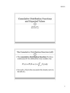
www.math.ttu.edu10/3/11 1 MATH 3342 SECTION 4.2 Cumulative Distribution Functions and Expected Values The Cumulative Distribution Function (cdf) ! The cumulative distribution function F(x) for a continuous RV X is defined for every number x by: For each x, F(x) is the area under the density curve to the left of x. F(x)=P(X≤x)=f(y)dy −∞