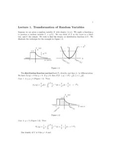
Lecture1.TransformationofRandomVariables
1. The joint density of two random variables X 1 and X 2 is f(x 1,x 2)=2e−x 1e−x 2, where 0 <x 1 <x 2 <∞;f(x 1,x 2) = 0 elsewhere. Consider the transformation Y 1 =2X 1,Y 2 = X 2 −X 1. Find the joint density of Y 1 and Y 2,and conclude thatY 1 and Y 2 are independent. 2. Repeat Problem 1 with the following new data. The joint density is ...
Download Lecture1.TransformationofRandomVariables

Information
Domain:
Source:
Link to this page:
Documents from same domain

Mathematical Logic (Math 570) Lecture Notes
faculty.math.illinois.edu2 CHAPTER 1. PRELIMINARIES all of mathematics. This era did not produce theorems in mathematical logic of any real depth, 1 but it did bring crucial progress of a conceptual nature, and the recognition that logic as used in mathematics obeys mathematical rules

Math 408, Spring 2008 Midterm Exam 2 Solutions
faculty.math.illinois.eduMath 408 Midterm Exam 2 Spring 2008 (b) Find the probability that the amount of the second claim is at least twice that of the first claim. Solution. Let X 1 and X 2 denote, respectively, the first and second claims. Then we need to compute P(X 2 …

Math 370/408, Spring 2008 Prof. A.J. Hildebrand Actuarial ...
faculty.math.illinois.eduMath 370/408 Spring 2008 Actuarial Exam Practice Problem Set 2 Solutions 1. [2-1] An insurance policy pays an individual 100 per day for up to 3 days of hospitalization and 25 per day for each day of hospitalization thereafter. The number of days of hospitalization, X, is a discrete random variable with probability function P(X = k) = (6−k

Even/odd proofs: Practice problems Solutions
faculty.math.illinois.eduSince the sum of two odd numbers is even (by Problem 1), s+t = p2 is even. Hence p, must be even as well (by Problem 2). Therefore p = 2h for some h 2Z, by the de nition of an even integer. 2. Math 347 Worksheet on \Even/odd" Proofs Solutions A.J. Hildebrand
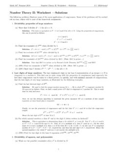
Number Theory II: Worksheet |Solutions
faculty.math.illinois.eduNext, we use the division algorithm to represent the given exponent 347 as a multiple of this (small) exponent we have found plus a remainder: 347 = 4 86 + 3: Finally, we use the properties of congruences and the fact that 34 1 mod 10 to nd the congruence sought: 3347 = 34 86+3 = (34)86 33 186 27 7 mod 10: Hence the last digit of 3347 in base ...

Math 220 Groupwok 10/12/17 Related Rates Word Problems
faculty.math.illinois.eduRelated Rates Word Problems SOLUTIONS (1)One car leaves a given point and travels north at 30 mph. Another car leaves 1 HOUR LATER, and travels west at 40 mph. At what rate is the distance between the cars changing at the instant the second car has been traveling for 1 hour? z x y Set up the problem by extracting information in terms of the ...
An Introduction to Complex Analysis and Geometry
faculty.math.illinois.eduOrthogonal trajectories and harmonic functions 97 5. A glimpse at harmonic functions 98 ... We de ne the exponential function by its power series and the cosine and sine functions by way of the exponential function. We can and therefore ... We also include sections on the Fourier transform on the Gamma function.
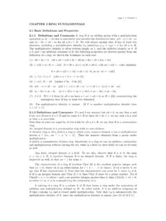
CHAPTER 2 RING FUNDAMENTALS 2.1 Basic Definitions and ...
faculty.math.illinois.edupage 1 of Chapter 2 CHAPTER 2 RING FUNDAMENTALS 2.1 Basic Definitions and Properties 2.1.1 Definitions and Comments A ringRis an abelian group with a multiplication operation (a,b) → abthat is associative and satisfies the distributive laws: a(b+c)=ab+acand (a+ b)c= ab+ acfor all a,b,c∈ R.We will always assume that Rhas at least two elements,including a multiplicative …
SECTION 1.6 FACTORING (Part II) FACTORING DIFFERENCE of ...
faculty.math.illinois.edu16 is a perfect square 16 can be written as 4 squared x is written as a factor twice Writing x2 as (x)2 shows this is a perfect square 25 is 5. 5 and a2 is a. a It is now rewritten as a square 9 is 3 3 and y4 could be written as It is now rewritten as a square > Quick check Write 64 and 9x4 each as a quantity squared.

GaloisTheory - University of Illinois Urbana-Champaign
faculty.math.illinois.eduGalois theory is based on a remarkable correspondence between subgroups of the Galois group of an extension E/Fand intermediate fields between Eand F. In this section we will set up the machinery for the fundamental theorem. [A remark on notation: Throughout the chapter,the compositionτ σof two automorphisms will be written as a product τσ.]
Related documents
Chapter 5: JOINT PROBABILITY DISTRIBUTIONS Part 1 ...
homepage.stat.uiowa.edudescribed with a joint probability mass function. If Xand Yare continuous, this distribution can be described with a joint probability density function. Example: Plastic covers for CDs (Discrete joint pmf) Measurements for the length and width of a rectangular plastic covers for CDs are rounded to the nearest mm(so they are discrete).
Chapter 5: JOINT PROBABILITY DISTRIBUTIONS Part 3: The ...
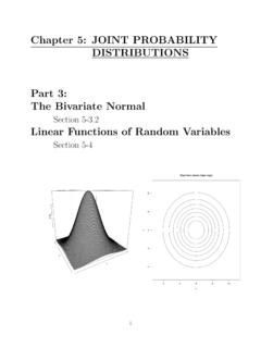
homepage.stat.uiowa.eduBivariate Normal Probability Density Function ... tour plot of the joint distribution looks like con-centric circles (or ellipses, if they have di erent variances) with major/minor axes that are par-allel/perpendicular to the x-axis: The center of each circle or …
Strict-Sense and Wide-Sense Stationarity Autocorrelation ...
isl.stanford.edu+sint with probability 1 4 −sint with probability 1 4 +cost with probability 1 4 −cost with probability 1 4 E(X(t)) = 0 and RX(t1,t2) = 1 2 cos(t2 −t1), thus X(t) is WSS But X(0) and X(π 4) do not have the same pmf (different ranges), so the first order pmf is not stationary, and the process is not SSS

Condit Density - Department of Statistics and Data Science
www.stat.yale.eduThe joint density for (X;Y) equals f(x;y) = (2ˇ) 1 exp (x2 + y2)=2. To nd the conditional density for Xgiven R= r, rst I’ll nd the joint density for Xand R, then I’ll calculate its Xmarginal, and then I’ll divide to get the conditional density. A simpler method is described at the end of the Example. We need to calculate Pfx 0 X x 0 + ;r ...
Probability, Statistics, and Random Processes for ...
www.sze.hu4.2 The Probability Density Function 148 4.3 The Expected Value of X 155 4.4 Important Continuous Random Variables 163 4.5 Functions of a Random Variable 174 4.6 The Markov and Chebyshev Inequalities 181 ... 5.3 The Joint cdf of X and Y 242 5.4 The Joint pdf of Two Continuous Random Variables 248
Exam 1 Practice Questions I - MIT OpenCourseWare
ocw.mit.edualways X minutes late, where X is an exponential random variable with probability density function f. X (x) = λe −λx. Suppose that you arrive at the bus stop precisely at noon. (a) Compute the probability that you have to wait for more than five minutes for the bus to arrive. (b) Suppose that you have already waiting for 10 minutes.

LECTURE NOTES on PROBABILITY and STATISTICS Eusebius …
users.encs.concordia.caJoint distributions 150 Marginal density functions 153 Independent continuous random variables 158 Conditional distributions 161 Expectation 163 Variance 169 Covariance 175 Markov’s inequality 181 ... The probability of a sequence to contain precisely two Heads is …
Conditional Joint Distributions
web.stanford.eduA joint probability density functiongives the relative likelihood of more than one continuous random variable each taking on a specific value. < £ < £ = ò ò 2 1 2 1 P(1 2, 1 2) , ( , ) a a b b a X a b Y b f X Y x y dy dx Joint Probability Density Function 0 y x 900 900 0 900 900
Lecture 5: Estimation
www.gs.washington.eduThe likelihood is the probability of the data given the parameter and represents the data now available. The prior is the probability of the parameter and represents what was