
Multivariate Data Analysis
1. Inertia: Trace(VQ) = Trace(WD) (inertia in the sense of Huyghens inertia formula for instance). Huygens,C. (1657), ∑n i=1 pid 2(x i;a) Inertia with regards to a pointaof a cloud ofpi-weighted points. PCAwithQ= Ip,D= 1 nIn,and the variables are centered,the inertia is the sum of the variances of all the variables.
Download Multivariate Data Analysis

Information
Domain:
Source:
Link to this page:
Documents from same domain
Chemical Engineering 160/260 Important …
web.stanford.eduChemical Engineering 160/260 Important Concepts, Lecture 9-16 Lecture 9: Introduction to Thermodynamic Models for Polymer/Solvent (and Polymer/Polymer

Game Review | The Legend of Zelda
web.stanford.eduTech Specs: like nuthin' your mama has ever seen. Two chip technologies in particular are responsible for LoZ's technological prowess: MMC (Memory
Assignment 1: Game Review “The Legend of Zelda”
web.stanford.eduNitin Chopra Assignment 1: Game Review “The Legend of Zelda” 1. Identify the Game I have chosen to do my Game Review on “The Legend of Zelda” because I …
Lecture 12 Feedback control systems: static analysis
web.stanford.eduLecture 12 Feedback control systems: ... sensors: radar altimeter; ... Feedback control systems: static analysis 12{4. Example
Credit Risk Modeling with Affine Processes
web.stanford.educredit-risk modeling (emphasizing the valuation of corporate debt and credit derivatives) with an introduction to the analytical tractability and richness of affine state processes. This is not a general survey of either topic, but rather

OBIEE Upgrade from 11G Oracle Business …
web.stanford.eduOracle Business Intelligence 12c is a unique platform that enables customers to uncover new insights and make faster, ... Oracle BI Enterprise Edition ...
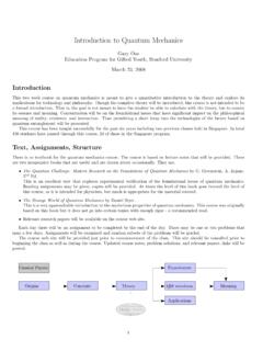
Introduction to Quantum Mechanics - Stanford …
web.stanford.eduIntroduction to Quantum Mechanics Gary Oas Education Program for Gifted Youth, Stanford University March 23, 2008 Introduction This two week course on quantum mechanics is meant to give a quantitative introduction to the theory and explore its
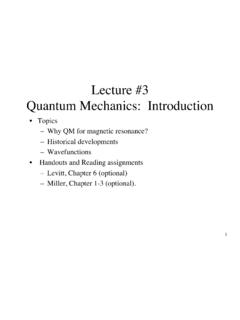
Lecture #3 Quantum Mechanics: Introduction
web.stanford.edu2 Classical versus Quantum NMR • QM is only theory that correctly predicts behavior of matter on the atomic scale, and QM effects are seen in vivo.
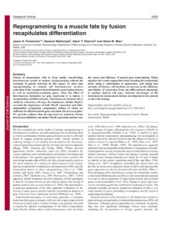
Reprogramming to a muscle fate by fusion …
web.stanford.eduResearch Article 1045 Introduction We have extended our earlier studies of nuclear reprogramming in heterokaryons to enhance our understanding of the mechanistic basis
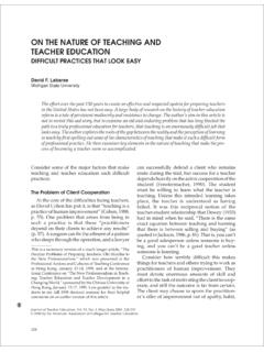
Journal of Teacher Education, Vol. 51, No. 3, …
web.stanford.eduON THE NATURE OF TEACHING AND TEACHER EDUCATION ... isolation is to create a vision of learning to teach as a private ordeal (Lortie, 1975) and a vision of
Related documents
TIME SERIES - University of Cambridge
www.statslab.cam.ac.uk1 Models for time series 1.1 Time series data A time series is a set of statistics, usually collected at regular intervals. Time series data occur naturally in many application areas.

1 Multivariate Normal Distribution - Princeton University
www.cs.princeton.edu1 Multivariate Normal Distribution The multivariate normal distribution (MVN), also known as multivariate gaussian, is a generalization of the one-dimensional normal distribution to higher dimensions. The probability density function (pdf) of an MVN for a random vector x2Rd as follows: N(xj ;) , 1 (2ˇ)d=2j j1=2 exp 1 2 (x )T 1(x ) (1)

General Bivariate Normal - Duke University
www2.stat.duke.eduMatrix notation allows us to easily express the density of the multivariate normal distribution for an arbitrary number of dimensions. We express the k-dimensional multivariate normal distribution as follows, X ˘N k( ; There is a similar method for the multivariate normal distribution that) where is the k 1 column vector of means and is the k k

The Bivariate Normal Distribution - IIT Kanpur
home.iitk.ac.in2 The Bivariate Normal Distribution has a normal distribution. The reason is that if we have X = aU + bV and Y = cU +dV for some independent normal random variables U and V,then Z = s1(aU +bV)+s2(cU +dV)=(as1 +cs2)U +(bs1 +ds2)V. Thus, Z is the sum of the independent normal random variables (as1 + cs2)U and (bs1 +ds2)V, and is therefore normal.A very important …
Stata: Software for Statistics and Data Science | Stata
www.stata.comThe communalities are assumed to be 1. ipf specifies that the iterated principal-factor method be used to analyze the correlation matrix. This reestimates the communalities iteratively. ml specifies the maximum-likelihood factor method, assuming multivariate normal observations.

Multivariate Analysis Homework 1 - Michigan State University
www.stt.msu.eduMultivariate Analysis Homework 1 A49109720 Yi-Chen Zhang March 16, 2018 4.2. Consider a bivariate normal population with 1 = 0, 2 = 2, ˙ 11 = 2, ˙ 22 = 1, and ˆ 12 = 0:5. (a)Write out the bivariate normal density.

5.8 Lagrange Multipliers - Pennsylvania State University
www.personal.psu.eduMultivariate Calculus; Fall 2013 S. Jamshidi 4. x4 +y4 +z4 =1 If x,y,z are nonzero, then we can consider Therefore, we have the following equations: 1. 1=2x2 2. 1=2y2 3. 1=2z2 4. x4 +y4 +z4 =1 Remember, we can only make this simplification if all the variables are nonzero!